Credit Card Anomaly Detection
H2O Isolation Forest
Credit Card Fraud Detection
Anonymized credit card transactions labeled as fraudulent or genuine.
Fraud is a growing concern for companies all over the globe. While there are many ways to fight and identify fraud, one method that is gaining increased attention is the use of unsupervised learning methods to detect anomalies within customer or transactions data. By analyzing customers or transactions relative to each other, we’re able to spot unusual observations.
Unsupervised methods
These methods are referred to as unsupervised because there is no historical information about fraudulent cases that is used to train the model.Instead, unsupervised methods are used to find anomalies by locating observations within the data set that are separated from other heavily populated areas of the data set.
The assumption behind this is that fraudulent behavior can often appear as anomalous within a data set. It should be noted that just because an observation is anomalous, it doesn’t mean it is fraudulent or of interest to the user. Similarly, fraudulent behavior can be disguised to be hidden within more regular types of behavior. However, without labeled training data, unsupervised learning is a good method to use to begin to identify deviant accounts or transactions.
Why might want to use unsupervised methods instead of supervised methods.
Trying to find new types of fraud that may not have been captured within the historical data. Fraud patterns can evolve or change and so it is important to constantly be searching for ways to identify new patterns as early as possible. If purely relying on supervised models built with historical data, these new patterns can be missed. However, since the unsupervised methods are not limited by the patterns present in the historical data, they can potentially identify these new patterns as they may represent behavior that is unusual or anomalous.
What is an anomaly and how to identify it?
- Anomalies are data points that are few and different. It has a pattern that appears to have different characteristics from a normal data point.
- Anomaly detection is a common data science problem where the goal is to identify odd or suspicious observations, events, or items in our data that might be indicative of some issues in our data collection process
Three fundamental approaches to detect anomalies are based on:
- Density
- Distance
- Isolation.
The real challenge in anomaly detection is to construct the right data model to separate outliers from noise and normal data.
Anomaly == Outlier == Deviant or Unsual Data Point
Loading the Data
Before we dive into the anomaly detection, let’s initialize the h2o cluster and load our data in. We will be using the credit card data set, which contains information on various properties of credit card transactions. There are 492 fraudulent and 284,807 genuine transactions, which makes the target class highly imbalanced. We will not use the label during the anomaly detection modeling, but we will use it during the evaluation of our anomaly detection.
credit_card_tbl <- vroom("data/creditcard.csv")Exploratory Data Analysis
Exploratory Data Analysis is an initial process of analysis, in which you can summarize characteristics of data such as pattern, trends, outliers, and hypothesis testing using descriptive statistics and visualization.
Credit card transactions(Fraud vs Non-fraud)
fraud_class <- credit_card_tbl %>%
  group_by(Classes) %>%
  summarize(Count = n()) %>%
  ggplot(aes(x=Classes, y=Count, fill = Classes)) +
  geom_col() +
  theme_tufte() +
  scale_fill_manual(values=c("#377EB8","#E41A1C")) +
  geom_text(aes(label = Count), size = 3, vjust = 1.2, color = "#FFFFFF") +
  theme(plot.title = element_text(face = "bold", hjust = 0.5)) +
  labs(title="Credit card transactions", x = "Classes", y = "Count")

fraud_class_percentage <- credit_card_tbl %>%
  group_by(Classes) %>%
  summarise(Count=n()) %>%
  mutate(percent = round(prop.table(Count),2) * 100) %>%
  ggplot(aes("", Classes, fill = Classes)) +
  geom_bar(width = 1, stat = "identity", color = "white") +
  theme_tufte() +
  scale_fill_manual(values=c("#377EB8","#E41A1C")) +
  coord_polar("y", start = 0) +
  ggtitle("Credit card transactions(%)") +
  theme(plot.title = element_text(face = "bold", hjust = 0.5)) +
  geom_text(aes(label = paste0(round(percent, 1), "%")), position = position_stack(vjust = 0.5), color = "white")

plot_grid(fraud_class, fraud_class_percentage, align="h", ncol=2)
Amount spend vs Fraud
g <- credit_card_tbl %>%
    select(Amount, Class) %>%
    ggplot(aes(Amount, fill = as.factor(Class))) +
    # geom_histogram() +
    geom_density(alpha = 0.3) +
    facet_wrap(~ Class, scales = "free_y", ncol = 1) +
    scale_x_log10(label = scales::dollar_format()) +
    scale_fill_tq() +
    theme_tq() +
    labs(title = "Fraud by Amount Spent",
         fill = "Fraud")

ggplotly(g)
Isolation Forest
Let’s understand in detail what isolation forest is and how it can be helpful in identifying the anomaly.
The term isolation means separating an instance from the rest of the instances. Since anomalies are “few and different” and therefore they are more susceptible to isolation.
- Isolation Forest is an outlier detection technique that identifies anomalies instead of normal observations
- It identifies anomalies by isolating outliers in the data. Isolation forest exists under an unsupervised machine learning algorithm.and therefore it does not need labels to identify the outlier/anomaly.
Advantages of using Isolation Forest:
- One of the advantages of using the isolation forest is that it not only detects anomalies faster but also requires less memory compared to other anomaly detection algorithms.
- It can be scaled up to handle large, high-dimensional datasets.
First, we need to initialize the Java Virtual Machine (JVM) that H2O uses locally.
h2o.init()Next, we change our data to an h2o object that the package can interpret.
credit_card_h2o <- as.h2o(credit_card_tbl)target <- "Class"
predictors <- setdiff(names(credit_card_h2o), target)
# Let’s train isolation forest.
isoforest <- h2o.isolationForest(
training_frame = credit_card_h2o,
x = predictors,
ntrees = 100,
seed = 1234
)##
|
| | 0%
|
|= | 1%
|
|== | 3%
|
|===== | 7%
|
|======== | 11%
|
|=========== | 16%
|
|=============== | 21%
|
|=================== | 27%
|
|======================= | 33%
|
|============================ | 40%
|
|=============================== | 44%
|
|=================================== | 50%
|
|======================================= | 56%
|
|=========================================== | 61%
|
|=============================================== | 67%
|
|================================================== | 72%
|
|======================================================= | 78%
|
|========================================================== | 83%
|
|============================================================== | 88%
|
|================================================================== | 94%
|
|======================================================================| 100%isoforest## Model Details:
## ==============
##
## H2OAnomalyDetectionModel: isolationforest
## Model ID: IsolationForest_model_R_1615735708480_1
## Model Summary:
## number_of_trees number_of_internal_trees model_size_in_bytes min_depth
## 1 100 100 70553 8
## max_depth mean_depth min_leaves max_leaves mean_leaves
## 1 8 8.00000 15 94 51.48000
##
##
## H2OAnomalyDetectionMetrics: isolationforest
## ** Reported on training data. **
## ** Metrics reported on Out-Of-Bag training samples **Prediction
We can see that the prediction h2o frame contains two columns:
- predict: The likelihood of the observations being outlier.
- mean_length: Showing the average number of splits across all trees to isolate the observation.
predictions <- predict(isoforest, newdata = credit_card_h2o)##
|
| | 0%
|
|======================================================================| 100%predictions## predict mean_length
## 1 0.04724409 6.82
## 2 0.04986877 6.81
## 3 0.16010499 6.39
## 4 0.11023622 6.58
## 5 0.06561680 6.75
## 6 0.04986877 6.81
##
## [284807 rows x 2 columns]Metrics
Predicting Anomalies using Quantile
How do we go from the average number of splits / anomaly score to the actual predictions? Using a threshold If we have an idea about the relative number of outliers in our dataset, we can find the corresponding quantile value of the score and use it as a threshold for our predictions.
We can see that most of the observations are low percentage likelihood, but there are some with high likelihood and that is anomaly.
h2o.hist(predictions[,"predict"])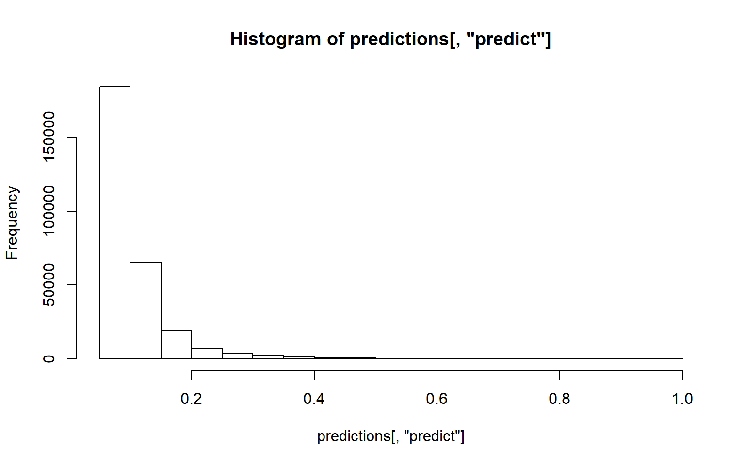
Most of the observations are around 7 trees / splits to be able separate the data points.
h2o.hist(predictions[,"mean_length"])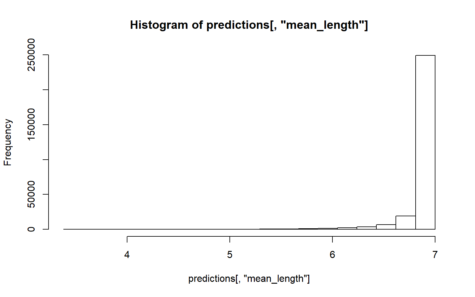
quantile <- h2o.quantile(predictions, probs = 0.99)
quantile## predictQuantiles mean_lengthQuantiles
## 0.3412073 7.0000000thresh <- quantile["predictQuantiles"]
predictions$outlier <- predictions$predict > thresh %>% as.numeric()
predictions$class <- credit_card_h2o$Class
predictions## predict mean_length outlier class
## 1 0.04724409 6.82 0 0
## 2 0.04986877 6.81 0 0
## 3 0.16010499 6.39 0 0
## 4 0.11023622 6.58 0 0
## 5 0.06561680 6.75 0 0
## 6 0.04986877 6.81 0 0
##
## [284807 rows x 4 columns]predictions_tbl <- as_tibble(predictions) %>%
mutate(class = factor(class, levels = c("1","0"))) %>%
mutate(outlier = factor(outlier,levels = c("1","0")))
predictions_tbl## # A tibble: 284,807 x 4
## predict mean_length outlier class
## <dbl> <dbl> <fct> <fct>
## 1 0.0472 6.82 0 0
## 2 0.0499 6.81 0 0
## 3 0.160 6.39 0 0
## 4 0.110 6.58 0 0
## 5 0.0656 6.75 0 0
## 6 0.0499 6.81 0 0
## 7 0.0551 6.79 0 0
## 8 0.168 6.36 0 0
## 9 0.0971 6.63 0 0
## 10 0.0525 6.8 0 0
## # ... with 284,797 more rowsConfusion Matrix
We have 300 anomalies which are considered as Fraud.
predictions_tbl %>% conf_mat(class, outlier)## Truth
## Prediction 1 0
## 1 300 2511
## 0 192 281804ROC Curve
auc <- predictions_tbl %>%
roc_auc(class, predict) %>%
pull(.estimate) %>%
round(3)
predictions_tbl %>%
roc_curve(class, predict) %>%
ggplot(aes(x = 1 - specificity, y = sensitivity)) +
geom_path(color = palette_light()[1], size = 2) +
geom_abline(lty = 3, size = 1) +
theme_tq() +
labs(title = str_glue("ROC AUC: {auc}"),
subtitle = "Using H2O Isolation Forest")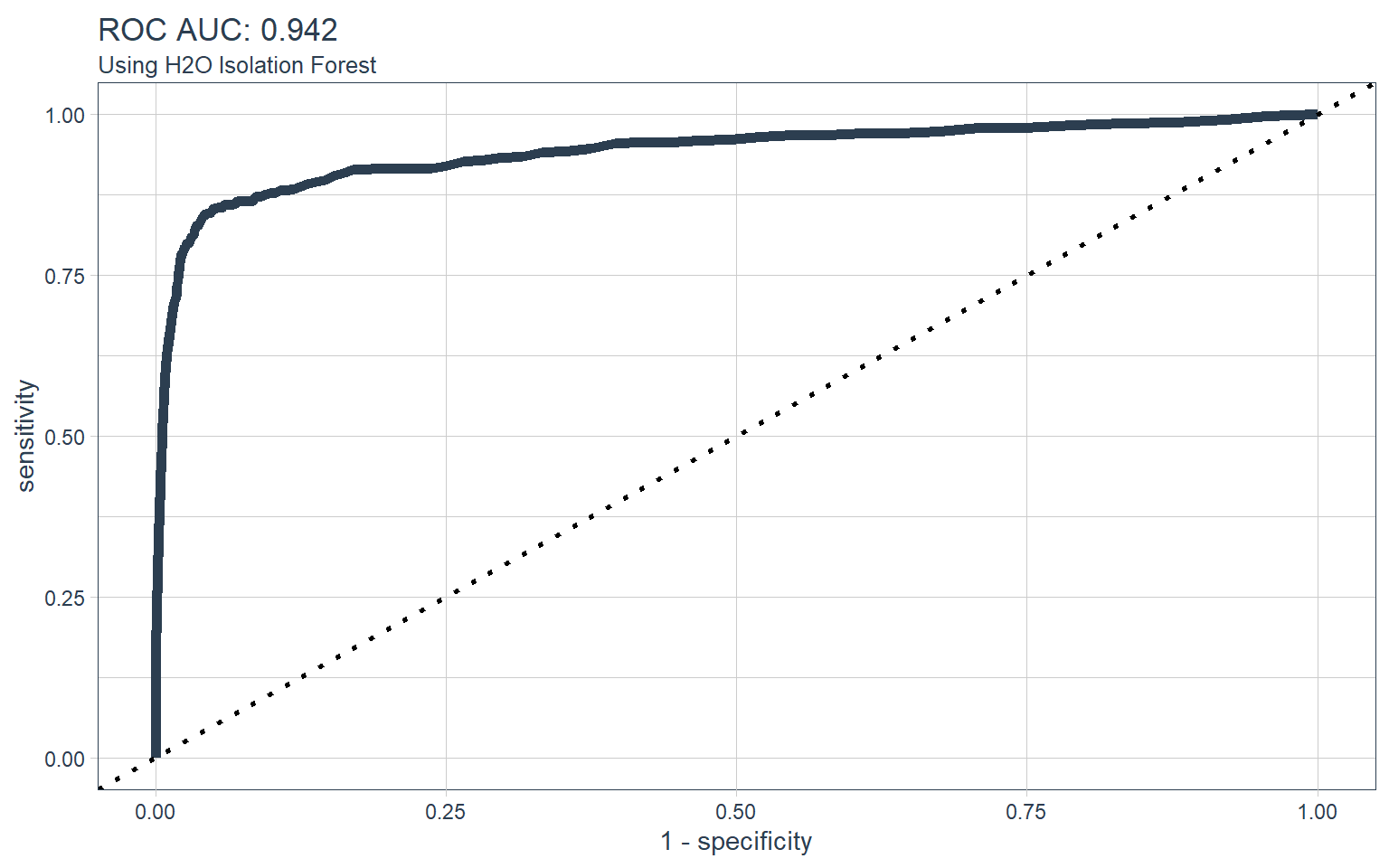
Stabilize Predictions
Stabilize predictions to increase anomaly detection performance
- Run algorithm multiple times, change seed parameter and average the results to stabilize..
- Adjust quantile / threshold based on visualizing outliers.
# Repeatable Prediction Function
iso_forest <- function(seed) {
target <- "Class"
predictors <- setdiff(names(credit_card_h2o), target)
isoforest <- h2o.isolationForest(
training_frame = credit_card_h2o,
x = predictors,
ntrees = 100,
seed = seed
)
predictions <- predict(isoforest, newdata = credit_card_h2o)
quantile <- h2o.quantile(predictions, probs = 0.99)
thresh <- quantile["predictQuantiles"]
# predictions$outlier <- predictions$predict > thresh %>% as.numeric()
# predictions$class <- credit_card_h2o$Class
predictions_tbl <- as_tibble(predictions) %>%
# mutate(class = as.factor(class)) %>%
mutate(row = row_number())
predictions_tbl
}iso_forest(123)##
|
| | 0%
|
|= | 2%
|
|==== | 5%
|
|======= | 10%
|
|=========== | 16%
|
|=============== | 22%
|
|==================== | 28%
|
|======================= | 33%
|
|=========================== | 39%
|
|================================ | 45%
|
|================================== | 48%
|
|==================================== | 52%
|
|======================================== | 57%
|
|=========================================== | 62%
|
|============================================== | 66%
|
|================================================== | 71%
|
|===================================================== | 76%
|
|========================================================= | 81%
|
|============================================================= | 87%
|
|================================================================ | 92%
|
|===================================================================== | 98%
|
|======================================================================| 100%
##
  |
  |                                                                      |   0%
  |
|======================================================================| 100%## # A tibble: 284,807 x 3
## predict mean_length row
## <dbl> <dbl> <int>
## 1 0.0431 6.83 1
## 2 0.0152 6.94 2
## 3 0.157 6.38 3
## 4 0.0533 6.79 4
## 5 0.0330 6.87 5
## 6 0.0203 6.92 6
## 7 0.00761 6.97 7
## 8 0.190 6.25 8
## 9 0.0457 6.82 9
## 10 0.0279 6.89 10
## # ... with 284,797 more rowsMap to multiple seeds
multiple_predictions_tbl <- tibble(seed = c(158, 8546, 4593)) %>%
mutate(predictions = map(seed, iso_forest))multiple_predictions_tbl## # A tibble: 3 x 2
## seed predictions
## <dbl> <list>
## 1 158 <tibble [284,807 x 3]>
## 2 8546 <tibble [284,807 x 3]>
## 3 4593 <tibble [284,807 x 3]>Precision vs Recall AUC
# Calculate average predictions
stabilized_predictions_tbl <- multiple_predictions_tbl %>%
    unnest(predictions) %>%
    select(row, seed, predict) %>%

    # Calculate stabilized predictions
    group_by(row) %>%
    summarize(mean_predict = mean(predict)) %>%
    ungroup() %>%

    # Combine with original data & important columns
    bind_cols(
        credit_card_tbl
    ) %>%
    select(row, mean_predict, Time, V12, V15, Amount, Class) %>%

    # Detect Outliers
    mutate(outlier = ifelse(mean_predict > quantile(mean_predict, probs = 0.99), 1, 0)) %>%
    mutate(Class = as.factor(Class))

stabilized_predictions_tbl %>% pr_auc(Class, mean_predict)
## # A tibble: 1 x 3
## .metric .estimator .estimate
## <chr> <chr> <dbl>
## 1 pr_auc binary 0.991stabilized_predictions_tbl %>%
ggplot(aes(V12, V15, color = as.factor(outlier))) +
geom_point(alpha = 0.2) +
theme_tq() +
scale_color_tq() +
labs(title = "Anomaly Detected?", color = "Is Outlier?")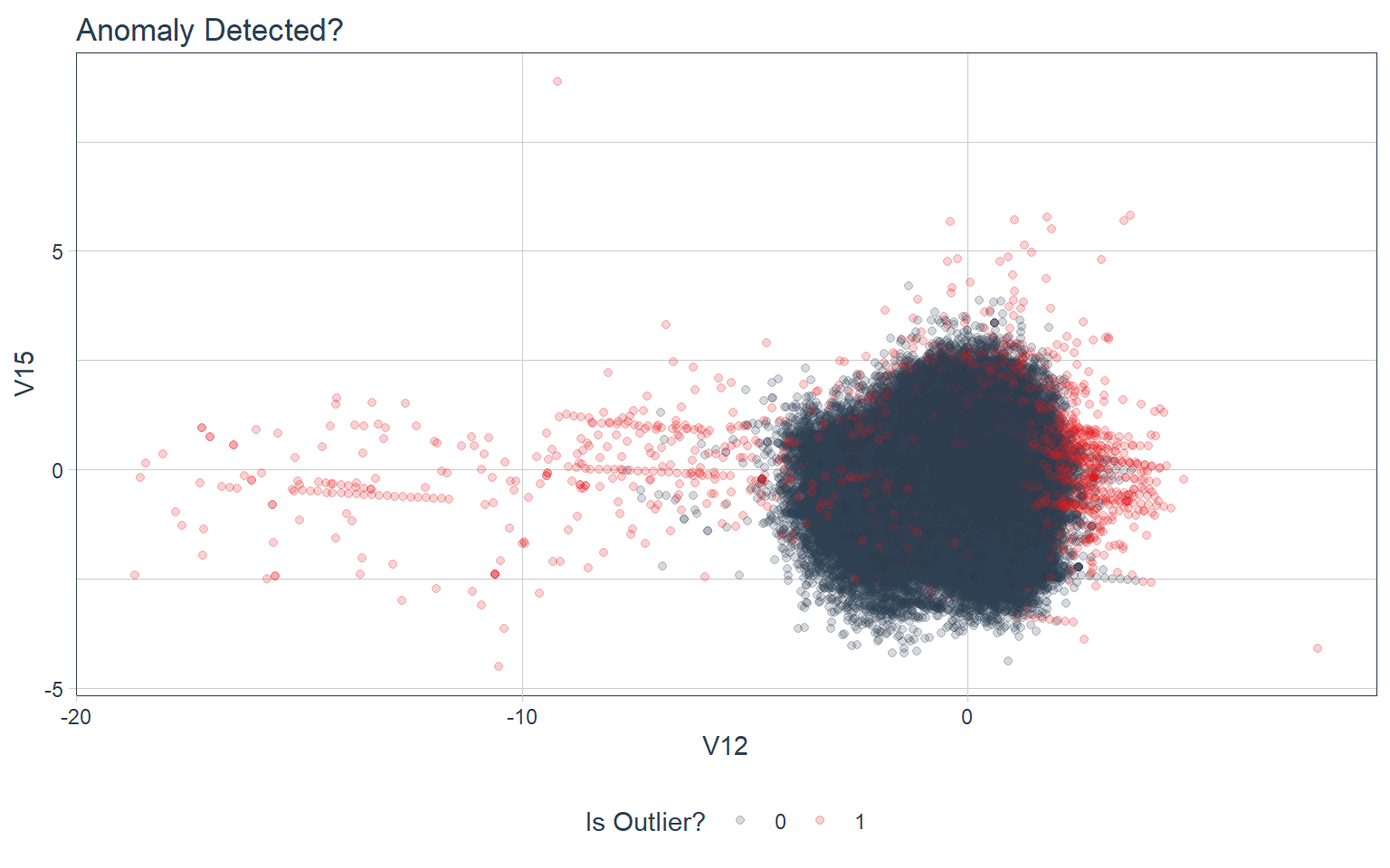
stabilized_predictions_tbl %>%
    ggplot(aes(V12, V15, color = as.factor(outlier))) +
    geom_point(alpha = 0.2) +
    theme_tq() +
    scale_color_tq() +
    labs(title = "Fraud Present?", color = "Is Fraud?")
Conclusions
- Anomalies (Outliers) are more often than not Fraudulent Transactions.
- Isolation Forest does a good job at detecting anomalous behaviour.