Customer Community Network Detection.

Business Understanding

As marketers, we often fall into the trap of trying to please everyone. This is a massive mistake that can end in disaster. What if there was a way to customize products to a specific group of people and have them go viral?

Understanding the strength of the relationship and which customers are more important to analyze.
How to use Network Analysis to identify the most influential customer networks within your customer-base. It’s then easy to cater products to them. The result is that products are much more likely to go viral!
Increase your customer segmentation explainability

Network Analysis

Community Detection

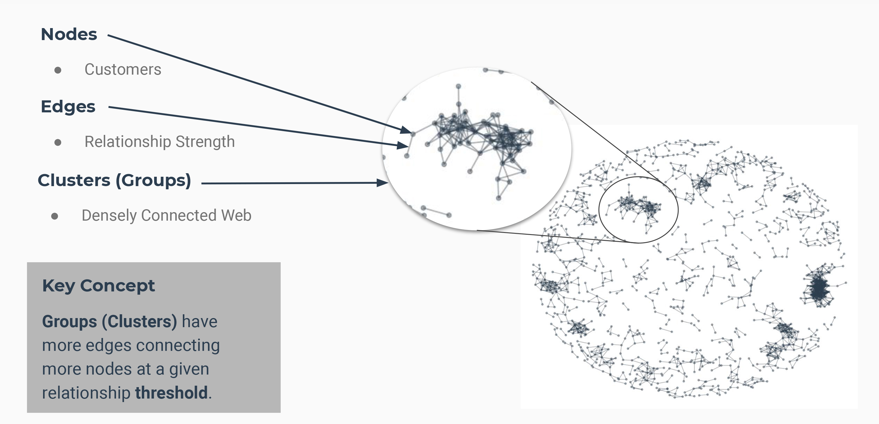
Community Detection is one of the fundamental problems in network analysis, where the goal is to find groups of nodes that are, in some sense, more similar to each other than to the other nodes.

Communities or clusters are usually groups of vertices having higher probability of being connected to each other than to members of other groups.

Network Types

There are two types of network Analysis:

Undirected Strength of Relationship
Directed Hierarchical Structure

I will be using Undirected (Strength of Relationship) for Clustering.

Preparations

Load libraries

library(tidyverse)
library(tidyquant)

# EDA
library(DataExplorer)
library(correlationfunnel)

# Pre-processing
library(recipes)

# Network Analysis
library(tidygraph)
library(ggraph)

library(knitr)

Data

credit_card_tbl <- read_csv("data/CC GENERAL.csv")

Glimpse

credit_card_tbl %>% glimpse()

## Rows: 8,950
## Columns: 18
## $ CUST_ID                          <chr> "C10001", "C10002", "C10003", "C10...
## $ BALANCE                          <dbl> 40.90075, 3202.46742, 2495.14886, ...
## $ BALANCE_FREQUENCY                <dbl> 0.818182, 0.909091, 1.000000, 0.63...
## $ PURCHASES                        <dbl> 95.40, 0.00, 773.17, 1499.00, 16.0...
## $ ONEOFF_PURCHASES                 <dbl> 0.00, 0.00, 773.17, 1499.00, 16.00...
## $ INSTALLMENTS_PURCHASES           <dbl> 95.40, 0.00, 0.00, 0.00, 0.00, 133...
## $ CASH_ADVANCE                     <dbl> 0.0000, 6442.9455, 0.0000, 205.788...
## $ PURCHASES_FREQUENCY              <dbl> 0.166667, 0.000000, 1.000000, 0.08...
## $ ONEOFF_PURCHASES_FREQUENCY       <dbl> 0.000000, 0.000000, 1.000000, 0.08...
## $ PURCHASES_INSTALLMENTS_FREQUENCY <dbl> 0.083333, 0.000000, 0.000000, 0.00...
## $ CASH_ADVANCE_FREQUENCY           <dbl> 0.000000, 0.250000, 0.000000, 0.08...
## $ CASH_ADVANCE_TRX                 <dbl> 0, 4, 0, 1, 0, 0, 0, 0, 0, 0, 0, 0...
## $ PURCHASES_TRX                    <dbl> 2, 0, 12, 1, 1, 8, 64, 12, 5, 3, 1...
## $ CREDIT_LIMIT                     <dbl> 1000, 7000, 7500, 7500, 1200, 1800...
## $ PAYMENTS                         <dbl> 201.8021, 4103.0326, 622.0667, 0.0...
## $ MINIMUM_PAYMENTS                 <dbl> 139.50979, 1072.34022, 627.28479, ...
## $ PRC_FULL_PAYMENT                 <dbl> 0.000000, 0.222222, 0.000000, 0.00...
## $ TENURE                           <dbl> 12, 12, 12, 12, 12, 12, 12, 12, 12...

Customer Segmentation Workflow

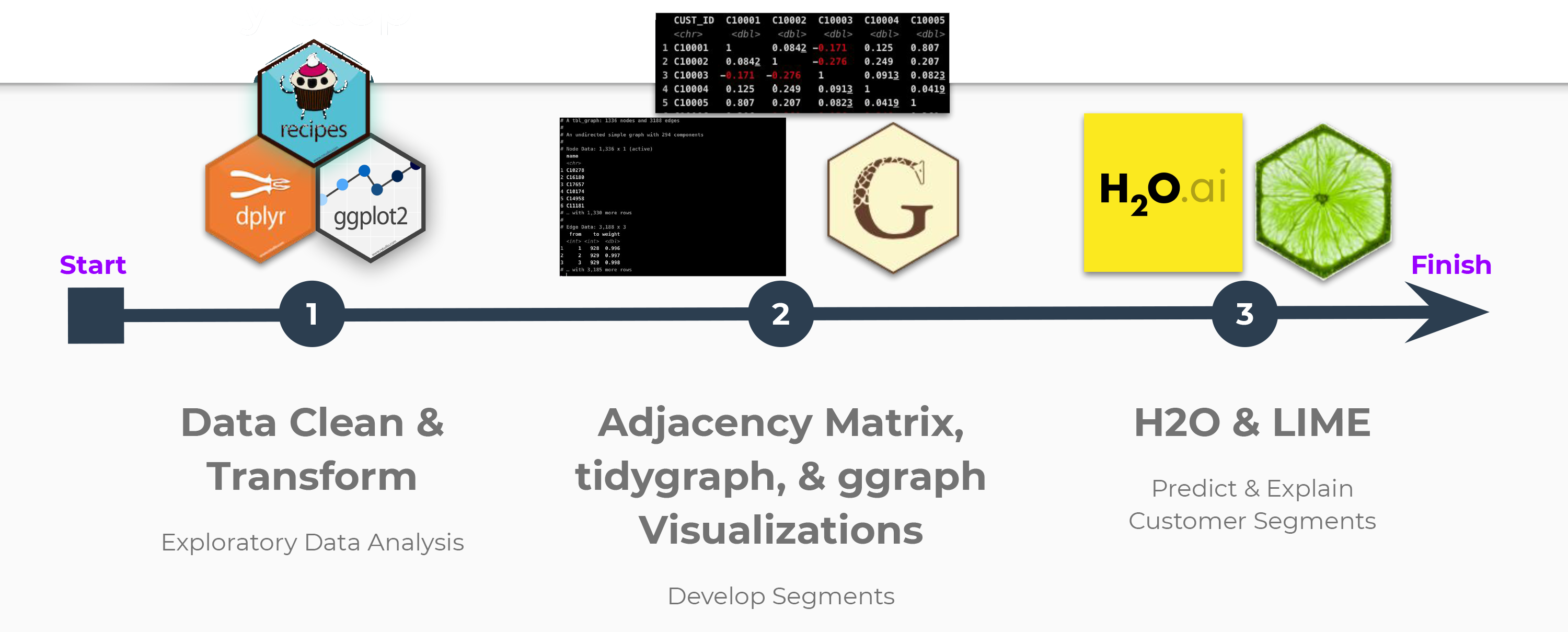
Exploratory Data Analysis (EDA)

plot_missing(credit_card_tbl)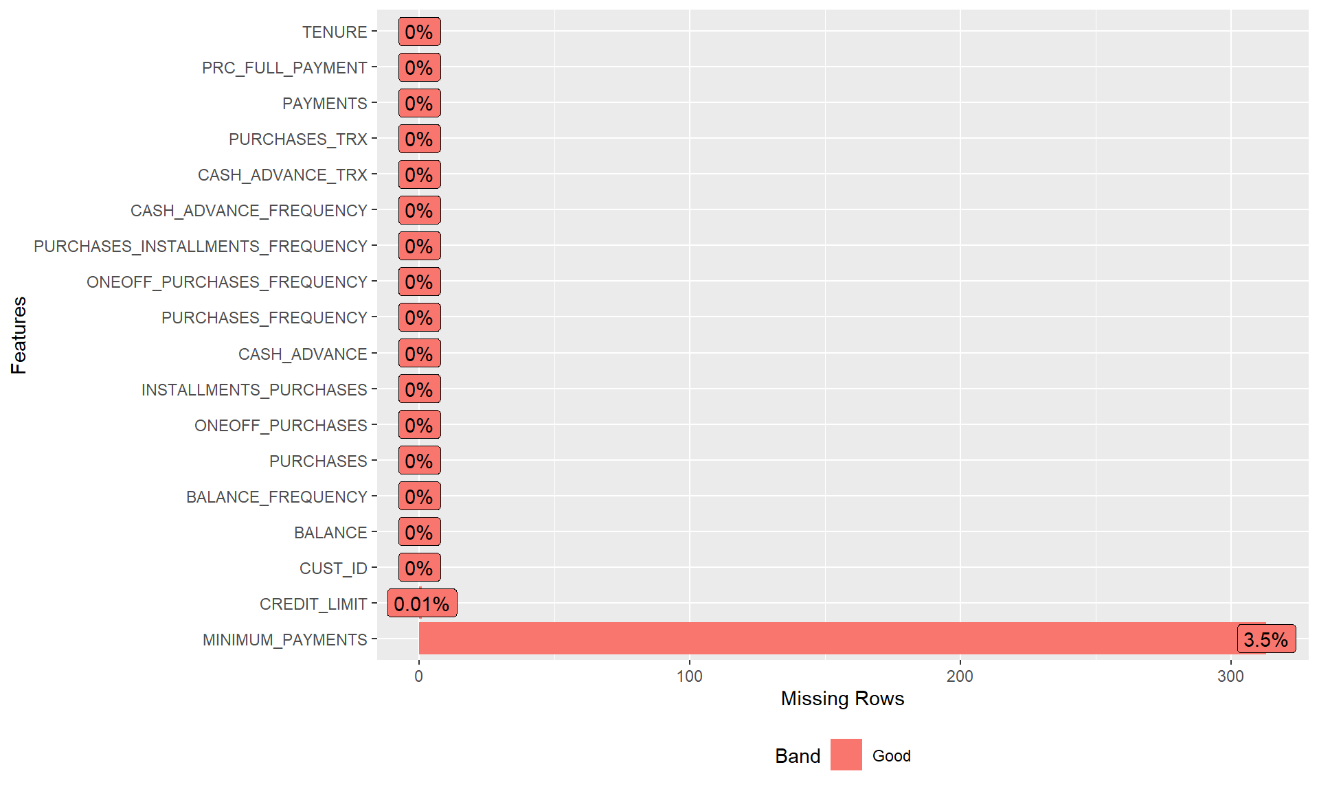

Missing Data

Minimum Payments

Minimum Payments has NA (missing data)

# Quantile 
credit_card_tbl %>%
    pull(MINIMUM_PAYMENTS) %>%
    quantile(na.rm = TRUE)

##           0%          25%          50%          75%         100% 
##     0.019163   169.123707   312.343947   825.485459 76406.207520

Correlation Funnel

# Filter all non-missing data
credit_card_no_missing_tbl <- credit_card_tbl %>%
    select_if(is.numeric) %>%
    filter(!is.na(MINIMUM_PAYMENTS)) %>%
    filter(!is.na(CREDIT_LIMIT)) 

credit_card_no_missing_tbl %>%
    binarize() %>%
    correlate(target = MINIMUM_PAYMENTS__825.49646275_Inf) %>% # Largest bin for minimum payment
    plot_correlation_funnel()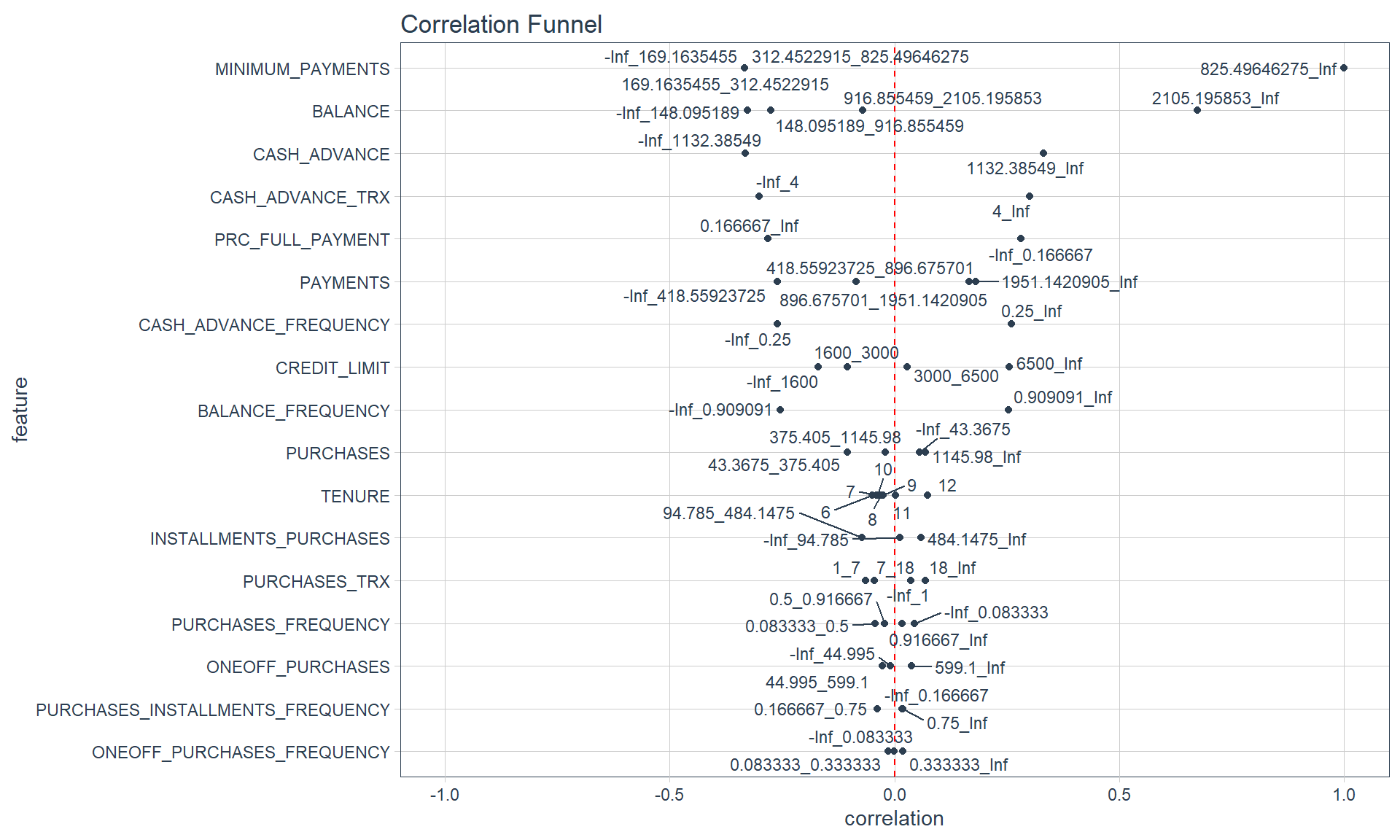

Linear Model (lm)

credit_card_tbl %>%
    ggplot(aes(BALANCE, MINIMUM_PAYMENTS)) + 
    geom_point(alpha = 0.25) +
    geom_smooth(method = "lm")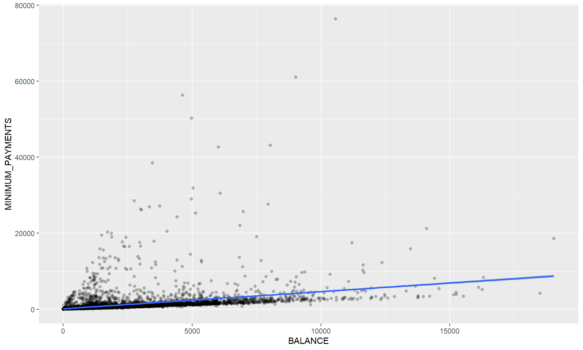

Credit Limit

Credit Limit has NA (missing data)

# Quantile
credit_card_tbl %>%
    pull(CREDIT_LIMIT) %>%
    quantile(na.rm = TRUE)

##    0%   25%   50%   75%  100% 
##    50  1600  3000  6500 30000

Correlation Funnel

credit_card_no_missing_tbl %>%
    binarize() %>%
    correlate(target = CREDIT_LIMIT__6500_Inf) %>% # Largest credit limit bin
    plot_correlation_funnel()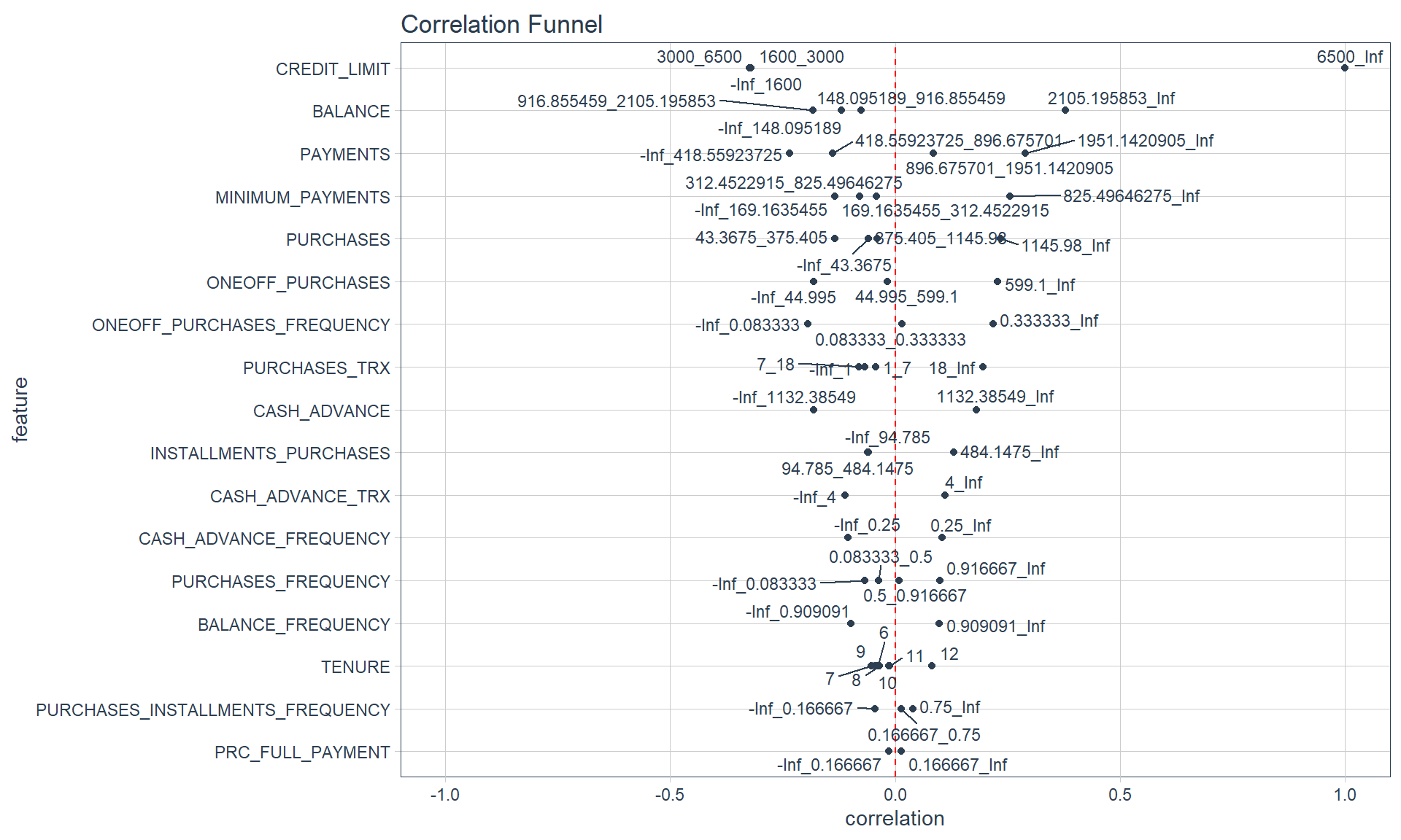

Linear Model (lm)

credit_card_tbl %>%
  ggplot(aes(BALANCE, CREDIT_LIMIT)) + 
  geom_point(alpha = 0.25) +
  geom_smooth(method = "lm")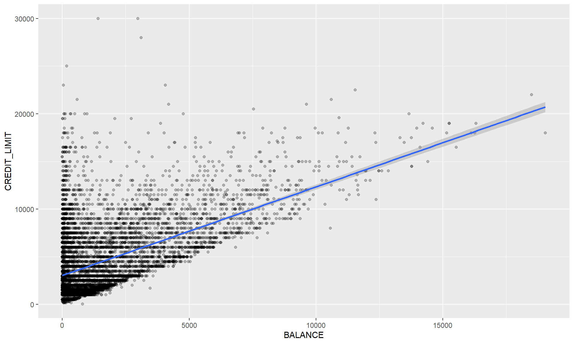

Pre-processing

Imputation and Standardized

rec_obj <- recipe(~ ., data = credit_card_tbl) %>%
    # Random Forest Imputation
    step_bagimpute(MINIMUM_PAYMENTS, CREDIT_LIMIT) %>%
    # Scale & Center for relationship analysis           
    step_center(all_numeric()) %>%
    step_scale(all_numeric()) %>%
    prep()

train_tbl <- bake(rec_obj, new_data = credit_card_tbl)
train_tbl

## # A tibble: 8,950 x 18
##    CUST_ID BALANCE BALANCE_FREQUEN~ PURCHASES ONEOFF_PURCHASES INSTALLMENTS_PU~
##    <fct>     <dbl>            <dbl>     <dbl>            <dbl>            <dbl>
##  1 C10001  -0.732            -0.249   -0.425           -0.357           -0.349 
##  2 C10002   0.787             0.134   -0.470           -0.357           -0.455 
##  3 C10003   0.447             0.518   -0.108            0.109           -0.455 
##  4 C10004   0.0491           -1.02     0.232            0.546           -0.455 
##  5 C10005  -0.359             0.518   -0.462           -0.347           -0.455 
##  6 C10006   0.118             0.518    0.154           -0.357            1.02  
##  7 C10007  -0.450             0.518    2.85             3.50             0.307 
##  8 C10008   0.125             0.518   -0.265           -0.357            0.0278
##  9 C10009  -0.264             0.518   -0.0663           0.0416          -0.233 
## 10 C10010  -0.678            -1.40     0.130            0.415           -0.455 
## # ... with 8,940 more rows, and 12 more variables: CASH_ADVANCE <dbl>,
## #   PURCHASES_FREQUENCY <dbl>, ONEOFF_PURCHASES_FREQUENCY <dbl>,
## #   PURCHASES_INSTALLMENTS_FREQUENCY <dbl>, CASH_ADVANCE_FREQUENCY <dbl>,
## #   CASH_ADVANCE_TRX <dbl>, PURCHASES_TRX <dbl>, CREDIT_LIMIT <dbl>,
## #   PAYMENTS <dbl>, MINIMUM_PAYMENTS <dbl>, PRC_FULL_PAYMENT <dbl>,
## #   TENURE <dbl>

Adjacency Matrix

To compare all features to see what customers correlate or related together.

customer_correlation_matrix <- train_tbl %>%
    
    # Transpose data for customer similarity
    gather(key = "FEATURE", value = "value", -CUST_ID, factor_key = TRUE) %>%
    spread(key = CUST_ID, value = value) %>%
    select(-FEATURE) %>%
    
    # Adjacency Matrix - Perform Similarity using Correlation
    as.matrix() %>%
    cor()

Customer Correlation Matrix

This is adjacency matrix that show how every customers are correlated against the other customers. Relationshiop Between Each Customers

customer_correlation_matrix %>% as_tibble(rownames = "CUST_ID")

## # A tibble: 8,950 x 8,951
##    CUST_ID  C10001  C10002  C10003  C10004  C10005 C10006  C10007  C10008 C10009
##    <chr>     <dbl>   <dbl>   <dbl>   <dbl>   <dbl>  <dbl>   <dbl>   <dbl>  <dbl>
##  1 C10001   1       0.0842 -0.171   0.125   0.807   0.386 -0.193   0.0384 0.279 
##  2 C10002   0.0842  1      -0.276   0.249   0.207  -0.360 -0.444  -0.469  0.0102
##  3 C10003  -0.171  -0.276   1       0.0913  0.0823 -0.156  0.292  -0.0332 0.266 
##  4 C10004   0.125   0.249   0.0913  1       0.0420 -0.345  0.222  -0.496  0.464 
##  5 C10005   0.807   0.207   0.0823  0.0420  1       0.269 -0.221  -0.0653 0.434 
##  6 C10006   0.386  -0.360  -0.156  -0.345   0.269   1     -0.271   0.696  0.185 
##  7 C10007  -0.193  -0.444   0.292   0.222  -0.221  -0.271  1      -0.0878 0.214 
##  8 C10008   0.0384 -0.469  -0.0332 -0.496  -0.0653  0.696 -0.0878  1      0.125 
##  9 C10009   0.279   0.0102  0.266   0.464   0.434   0.185  0.214   0.125  1     
## 10 C10010  -0.0500  0.135   0.226   0.860  -0.168  -0.390  0.433  -0.440  0.508 
## # ... with 8,940 more rows, and 8,941 more variables: C10010 <dbl>,
## #   C10011 <dbl>, C10012 <dbl>, C10013 <dbl>, C10014 <dbl>, C10015 <dbl>,
## #   C10016 <dbl>, C10017 <dbl>, C10018 <dbl>, C10019 <dbl>, C10020 <dbl>,
## #   C10021 <dbl>, C10022 <dbl>, C10023 <dbl>, C10024 <dbl>, C10025 <dbl>,
## #   C10026 <dbl>, C10027 <dbl>, C10028 <dbl>, C10029 <dbl>, C10030 <dbl>,
## #   C10031 <dbl>, C10032 <dbl>, C10033 <dbl>, C10034 <dbl>, C10035 <dbl>,
## #   C10036 <dbl>, C10037 <dbl>, C10038 <dbl>, C10039 <dbl>, C10040 <dbl>,
## #   C10041 <dbl>, C10043 <dbl>, C10044 <dbl>, C10045 <dbl>, C10046 <dbl>,
## #   C10047 <dbl>, C10048 <dbl>, C10049 <dbl>, C10050 <dbl>, C10051 <dbl>,
## #   C10052 <dbl>, C10053 <dbl>, C10054 <dbl>, C10055 <dbl>, C10056 <dbl>,
## #   C10057 <dbl>, C10058 <dbl>, C10059 <dbl>, C10060 <dbl>, C10061 <dbl>,
## #   C10062 <dbl>, C10063 <dbl>, C10064 <dbl>, C10065 <dbl>, C10067 <dbl>,
## #   C10068 <dbl>, C10069 <dbl>, C10070 <dbl>, C10071 <dbl>, C10072 <dbl>,
## #   C10073 <dbl>, C10074 <dbl>, C10075 <dbl>, C10077 <dbl>, C10078 <dbl>,
## #   C10079 <dbl>, C10080 <dbl>, C10081 <dbl>, C10082 <dbl>, C10083 <dbl>,
## #   C10084 <dbl>, C10085 <dbl>, C10086 <dbl>, C10087 <dbl>, C10088 <dbl>,
## #   C10089 <dbl>, C10090 <dbl>, C10092 <dbl>, C10093 <dbl>, C10094 <dbl>,
## #   C10095 <dbl>, C10096 <dbl>, C10097 <dbl>, C10098 <dbl>, C10099 <dbl>,
## #   C10100 <dbl>, C10101 <dbl>, C10102 <dbl>, C10103 <dbl>, C10104 <dbl>,
## #   C10105 <dbl>, C10106 <dbl>, C10107 <dbl>, C10108 <dbl>, C10109 <dbl>,
## #   C10110 <dbl>, C10111 <dbl>, C10112 <dbl>, C10113 <dbl>, ...

Pruning The Adjacency Matrix

Remove customer relationships or related to themselves

diag(customer_correlation_matrix) <- 0
customer_correlation_matrix %>% as_tibble(rownames = "CUST_ID")

## # A tibble: 8,950 x 8,951
##    CUST_ID  C10001  C10002  C10003  C10004  C10005 C10006  C10007  C10008 C10009
##    <chr>     <dbl>   <dbl>   <dbl>   <dbl>   <dbl>  <dbl>   <dbl>   <dbl>  <dbl>
##  1 C10001   0       0.0842 -0.171   0.125   0.807   0.386 -0.193   0.0384 0.279 
##  2 C10002   0.0842  0      -0.276   0.249   0.207  -0.360 -0.444  -0.469  0.0102
##  3 C10003  -0.171  -0.276   0       0.0913  0.0823 -0.156  0.292  -0.0332 0.266 
##  4 C10004   0.125   0.249   0.0913  0       0.0420 -0.345  0.222  -0.496  0.464 
##  5 C10005   0.807   0.207   0.0823  0.0420  0       0.269 -0.221  -0.0653 0.434 
##  6 C10006   0.386  -0.360  -0.156  -0.345   0.269   0     -0.271   0.696  0.185 
##  7 C10007  -0.193  -0.444   0.292   0.222  -0.221  -0.271  0      -0.0878 0.214 
##  8 C10008   0.0384 -0.469  -0.0332 -0.496  -0.0653  0.696 -0.0878  0      0.125 
##  9 C10009   0.279   0.0102  0.266   0.464   0.434   0.185  0.214   0.125  0     
## 10 C10010  -0.0500  0.135   0.226   0.860  -0.168  -0.390  0.433  -0.440  0.508 
## # ... with 8,940 more rows, and 8,941 more variables: C10010 <dbl>,
## #   C10011 <dbl>, C10012 <dbl>, C10013 <dbl>, C10014 <dbl>, C10015 <dbl>,
## #   C10016 <dbl>, C10017 <dbl>, C10018 <dbl>, C10019 <dbl>, C10020 <dbl>,
## #   C10021 <dbl>, C10022 <dbl>, C10023 <dbl>, C10024 <dbl>, C10025 <dbl>,
## #   C10026 <dbl>, C10027 <dbl>, C10028 <dbl>, C10029 <dbl>, C10030 <dbl>,
## #   C10031 <dbl>, C10032 <dbl>, C10033 <dbl>, C10034 <dbl>, C10035 <dbl>,
## #   C10036 <dbl>, C10037 <dbl>, C10038 <dbl>, C10039 <dbl>, C10040 <dbl>,
## #   C10041 <dbl>, C10043 <dbl>, C10044 <dbl>, C10045 <dbl>, C10046 <dbl>,
## #   C10047 <dbl>, C10048 <dbl>, C10049 <dbl>, C10050 <dbl>, C10051 <dbl>,
## #   C10052 <dbl>, C10053 <dbl>, C10054 <dbl>, C10055 <dbl>, C10056 <dbl>,
## #   C10057 <dbl>, C10058 <dbl>, C10059 <dbl>, C10060 <dbl>, C10061 <dbl>,
## #   C10062 <dbl>, C10063 <dbl>, C10064 <dbl>, C10065 <dbl>, C10067 <dbl>,
## #   C10068 <dbl>, C10069 <dbl>, C10070 <dbl>, C10071 <dbl>, C10072 <dbl>,
## #   C10073 <dbl>, C10074 <dbl>, C10075 <dbl>, C10077 <dbl>, C10078 <dbl>,
## #   C10079 <dbl>, C10080 <dbl>, C10081 <dbl>, C10082 <dbl>, C10083 <dbl>,
## #   C10084 <dbl>, C10085 <dbl>, C10086 <dbl>, C10087 <dbl>, C10088 <dbl>,
## #   C10089 <dbl>, C10090 <dbl>, C10092 <dbl>, C10093 <dbl>, C10094 <dbl>,
## #   C10095 <dbl>, C10096 <dbl>, C10097 <dbl>, C10098 <dbl>, C10099 <dbl>,
## #   C10100 <dbl>, C10101 <dbl>, C10102 <dbl>, C10103 <dbl>, C10104 <dbl>,
## #   C10105 <dbl>, C10106 <dbl>, C10107 <dbl>, C10108 <dbl>, C10109 <dbl>,
## #   C10110 <dbl>, C10111 <dbl>, C10112 <dbl>, C10113 <dbl>, ...

Remove duplicate relationships

customer_correlation_matrix[upper.tri(customer_correlation_matrix)] <- 0
customer_correlation_matrix %>% as_tibble(rownames = "CUST_ID")

## # A tibble: 8,950 x 8,951
##    CUST_ID  C10001  C10002  C10003  C10004  C10005 C10006  C10007 C10008 C10009
##    <chr>     <dbl>   <dbl>   <dbl>   <dbl>   <dbl>  <dbl>   <dbl>  <dbl>  <dbl>
##  1 C10001   0       0       0       0       0       0      0       0      0    
##  2 C10002   0.0842  0       0       0       0       0      0       0      0    
##  3 C10003  -0.171  -0.276   0       0       0       0      0       0      0    
##  4 C10004   0.125   0.249   0.0913  0       0       0      0       0      0    
##  5 C10005   0.807   0.207   0.0823  0.0420  0       0      0       0      0    
##  6 C10006   0.386  -0.360  -0.156  -0.345   0.269   0      0       0      0    
##  7 C10007  -0.193  -0.444   0.292   0.222  -0.221  -0.271  0       0      0    
##  8 C10008   0.0384 -0.469  -0.0332 -0.496  -0.0653  0.696 -0.0878  0      0    
##  9 C10009   0.279   0.0102  0.266   0.464   0.434   0.185  0.214   0.125  0    
## 10 C10010  -0.0500  0.135   0.226   0.860  -0.168  -0.390  0.433  -0.440  0.508
## # ... with 8,940 more rows, and 8,941 more variables: C10010 <dbl>,
## #   C10011 <dbl>, C10012 <dbl>, C10013 <dbl>, C10014 <dbl>, C10015 <dbl>,
## #   C10016 <dbl>, C10017 <dbl>, C10018 <dbl>, C10019 <dbl>, C10020 <dbl>,
## #   C10021 <dbl>, C10022 <dbl>, C10023 <dbl>, C10024 <dbl>, C10025 <dbl>,
## #   C10026 <dbl>, C10027 <dbl>, C10028 <dbl>, C10029 <dbl>, C10030 <dbl>,
## #   C10031 <dbl>, C10032 <dbl>, C10033 <dbl>, C10034 <dbl>, C10035 <dbl>,
## #   C10036 <dbl>, C10037 <dbl>, C10038 <dbl>, C10039 <dbl>, C10040 <dbl>,
## #   C10041 <dbl>, C10043 <dbl>, C10044 <dbl>, C10045 <dbl>, C10046 <dbl>,
## #   C10047 <dbl>, C10048 <dbl>, C10049 <dbl>, C10050 <dbl>, C10051 <dbl>,
## #   C10052 <dbl>, C10053 <dbl>, C10054 <dbl>, C10055 <dbl>, C10056 <dbl>,
## #   C10057 <dbl>, C10058 <dbl>, C10059 <dbl>, C10060 <dbl>, C10061 <dbl>,
## #   C10062 <dbl>, C10063 <dbl>, C10064 <dbl>, C10065 <dbl>, C10067 <dbl>,
## #   C10068 <dbl>, C10069 <dbl>, C10070 <dbl>, C10071 <dbl>, C10072 <dbl>,
## #   C10073 <dbl>, C10074 <dbl>, C10075 <dbl>, C10077 <dbl>, C10078 <dbl>,
## #   C10079 <dbl>, C10080 <dbl>, C10081 <dbl>, C10082 <dbl>, C10083 <dbl>,
## #   C10084 <dbl>, C10085 <dbl>, C10086 <dbl>, C10087 <dbl>, C10088 <dbl>,
## #   C10089 <dbl>, C10090 <dbl>, C10092 <dbl>, C10093 <dbl>, C10094 <dbl>,
## #   C10095 <dbl>, C10096 <dbl>, C10097 <dbl>, C10098 <dbl>, C10099 <dbl>,
## #   C10100 <dbl>, C10101 <dbl>, C10102 <dbl>, C10103 <dbl>, C10104 <dbl>,
## #   C10105 <dbl>, C10106 <dbl>, C10107 <dbl>, C10108 <dbl>, C10109 <dbl>,
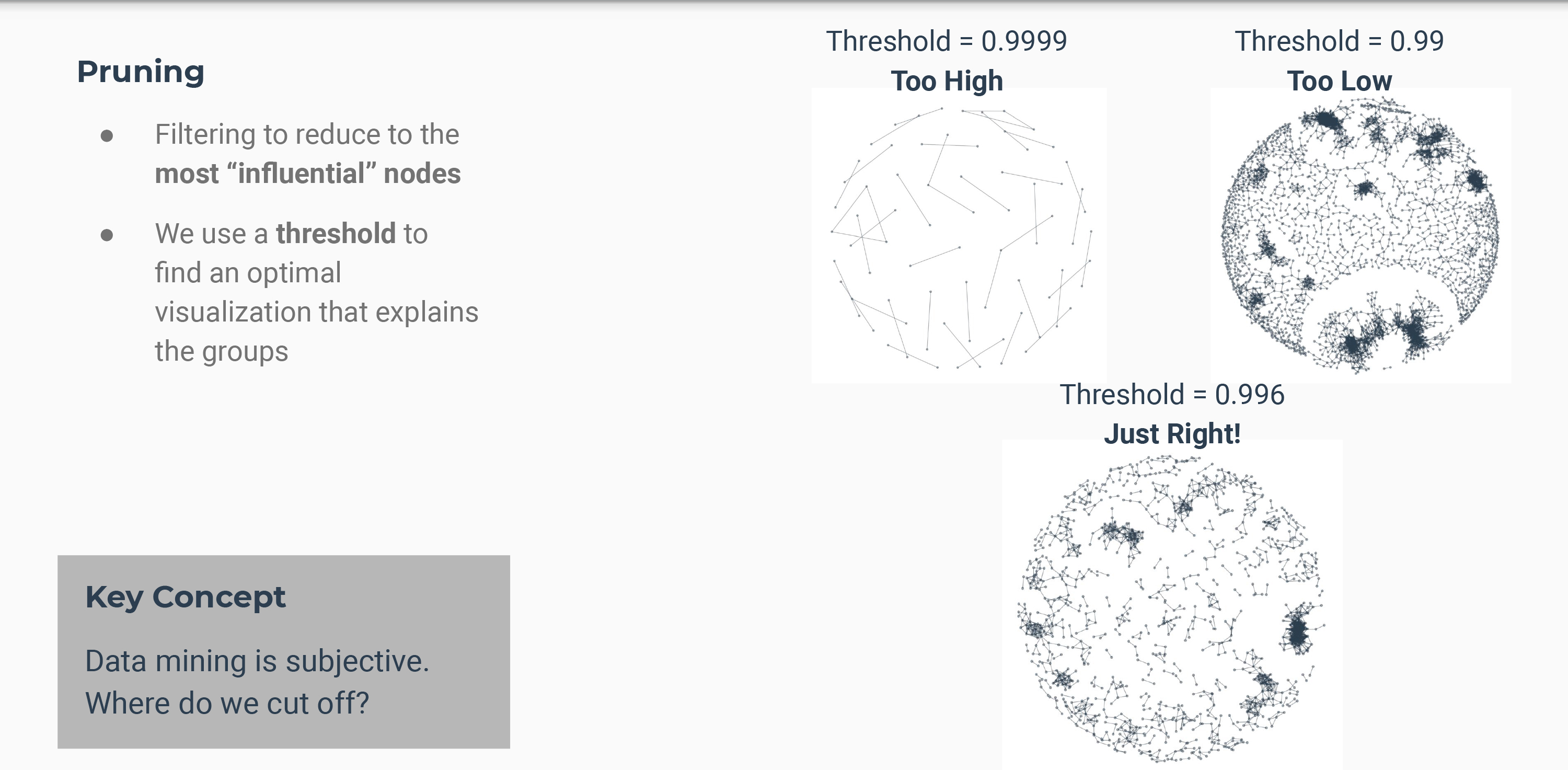
## #   C10110 <dbl>, C10111 <dbl>, C10112 <dbl>, C10113 <dbl>, ...

Prune relationships

Subsets of most influential customers.

edge_limit <- 0.99   # Below 0.99 gets zero values
customer_correlation_matrix[customer_correlation_matrix < edge_limit] <- 0
customer_correlation_matrix %>% as_tibble(rownames = "CUST_ID")

## # A tibble: 8,950 x 8,951
##    CUST_ID C10001 C10002 C10003 C10004 C10005 C10006 C10007 C10008 C10009 C10010
##    <chr>    <dbl>  <dbl>  <dbl>  <dbl>  <dbl>  <dbl>  <dbl>  <dbl>  <dbl>  <dbl>
##  1 C10001       0      0      0      0      0      0      0      0      0      0
##  2 C10002       0      0      0      0      0      0      0      0      0      0
##  3 C10003       0      0      0      0      0      0      0      0      0      0
##  4 C10004       0      0      0      0      0      0      0      0      0      0
##  5 C10005       0      0      0      0      0      0      0      0      0      0
##  6 C10006       0      0      0      0      0      0      0      0      0      0
##  7 C10007       0      0      0      0      0      0      0      0      0      0
##  8 C10008       0      0      0      0      0      0      0      0      0      0
##  9 C10009       0      0      0      0      0      0      0      0      0      0
## 10 C10010       0      0      0      0      0      0      0      0      0      0
## # ... with 8,940 more rows, and 8,940 more variables: C10011 <dbl>,
## #   C10012 <dbl>, C10013 <dbl>, C10014 <dbl>, C10015 <dbl>, C10016 <dbl>,
## #   C10017 <dbl>, C10018 <dbl>, C10019 <dbl>, C10020 <dbl>, C10021 <dbl>,
## #   C10022 <dbl>, C10023 <dbl>, C10024 <dbl>, C10025 <dbl>, C10026 <dbl>,
## #   C10027 <dbl>, C10028 <dbl>, C10029 <dbl>, C10030 <dbl>, C10031 <dbl>,
## #   C10032 <dbl>, C10033 <dbl>, C10034 <dbl>, C10035 <dbl>, C10036 <dbl>,
## #   C10037 <dbl>, C10038 <dbl>, C10039 <dbl>, C10040 <dbl>, C10041 <dbl>,
## #   C10043 <dbl>, C10044 <dbl>, C10045 <dbl>, C10046 <dbl>, C10047 <dbl>,
## #   C10048 <dbl>, C10049 <dbl>, C10050 <dbl>, C10051 <dbl>, C10052 <dbl>,
## #   C10053 <dbl>, C10054 <dbl>, C10055 <dbl>, C10056 <dbl>, C10057 <dbl>,
## #   C10058 <dbl>, C10059 <dbl>, C10060 <dbl>, C10061 <dbl>, C10062 <dbl>,
## #   C10063 <dbl>, C10064 <dbl>, C10065 <dbl>, C10067 <dbl>, C10068 <dbl>,
## #   C10069 <dbl>, C10070 <dbl>, C10071 <dbl>, C10072 <dbl>, C10073 <dbl>,
## #   C10074 <dbl>, C10075 <dbl>, C10077 <dbl>, C10078 <dbl>, C10079 <dbl>,
## #   C10080 <dbl>, C10081 <dbl>, C10082 <dbl>, C10083 <dbl>, C10084 <dbl>,
## #   C10085 <dbl>, C10086 <dbl>, C10087 <dbl>, C10088 <dbl>, C10089 <dbl>,
## #   C10090 <dbl>, C10092 <dbl>, C10093 <dbl>, C10094 <dbl>, C10095 <dbl>,
## #   C10096 <dbl>, C10097 <dbl>, C10098 <dbl>, C10099 <dbl>, C10100 <dbl>,
## #   C10101 <dbl>, C10102 <dbl>, C10103 <dbl>, C10104 <dbl>, C10105 <dbl>,
## #   C10106 <dbl>, C10107 <dbl>, C10108 <dbl>, C10109 <dbl>, C10110 <dbl>,
## #   C10111 <dbl>, C10112 <dbl>, C10113 <dbl>, C10114 <dbl>, ...

sum(customer_correlation_matrix > 0)

## [1] 10703

Filter relationships to subset of customers that have relationships

customer_correlation_matrix <- customer_correlation_matrix[rowSums(customer_correlation_matrix) > 0, colSums(customer_correlation_matrix) > 0] 
customer_correlation_matrix %>% dim()

## [1] 1992 1991

customer_correlation_matrix %>% as_tibble(rownames = "CUST_ID")

## # A tibble: 1,992 x 1,992
##    CUST_ID C10003 C10005 C10008 C10011 C10015 C10017 C10021 C10026 C10027 C10028
##    <chr>    <dbl>  <dbl>  <dbl>  <dbl>  <dbl>  <dbl>  <dbl>  <dbl>  <dbl>  <dbl>
##  1 C10102   0          0      0  0          0      0      0      0      0  0    
##  2 C10166   0          0      0  0          0      0      0      0      0  0    
##  3 C10174   0          0      0  0.997      0      0      0      0      0  0    
##  4 C10213   0          0      0  0          0      0      0      0      0  0    
##  5 C10256   0          0      0  0          0      0      0      0      0  0.996
##  6 C10278   0.996      0      0  0          0      0      0      0      0  0    
##  7 C10300   0          0      0  0          0      0      0      0      0  0    
##  8 C10321   0          0      0  0          0      0      0      0      0  0    
##  9 C10371   0          0      0  0          0      0      0      0      0  0    
## 10 C10391   0          0      0  0          0      0      0      0      0  0    
## # ... with 1,982 more rows, and 1,981 more variables: C10034 <dbl>,
## #   C10036 <dbl>, C10044 <dbl>, C10045 <dbl>, C10049 <dbl>, C10050 <dbl>,
## #   C10054 <dbl>, C10063 <dbl>, C10065 <dbl>, C10069 <dbl>, C10070 <dbl>,
## #   C10082 <dbl>, C10087 <dbl>, C10089 <dbl>, C10093 <dbl>, C10094 <dbl>,
## #   C10097 <dbl>, C10100 <dbl>, C10103 <dbl>, C10104 <dbl>, C10109 <dbl>,
## #   C10111 <dbl>, C10112 <dbl>, C10118 <dbl>, C10123 <dbl>, C10124 <dbl>,
## #   C10128 <dbl>, C10134 <dbl>, C10138 <dbl>, C10140 <dbl>, C10158 <dbl>,
## #   C10165 <dbl>, C10166 <dbl>, C10167 <dbl>, C10170 <dbl>, C10171 <dbl>,
## #   C10174 <dbl>, C10181 <dbl>, C10187 <dbl>, C10189 <dbl>, C10197 <dbl>,
## #   C10198 <dbl>, C10207 <dbl>, C10209 <dbl>, C10213 <dbl>, C10223 <dbl>,
## #   C10234 <dbl>, C10239 <dbl>, C10242 <dbl>, C10244 <dbl>, C10256 <dbl>,
## #   C10257 <dbl>, C10260 <dbl>, C10263 <dbl>, C10286 <dbl>, C10287 <dbl>,
## #   C10288 <dbl>, C10297 <dbl>, C10300 <dbl>, C10304 <dbl>, C10305 <dbl>,
## #   C10309 <dbl>, C10321 <dbl>, C10324 <dbl>, C10327 <dbl>, C10328 <dbl>,
## #   C10329 <dbl>, C10330 <dbl>, C10333 <dbl>, C10334 <dbl>, C10336 <dbl>,
## #   C10338 <dbl>, C10341 <dbl>, C10347 <dbl>, C10349 <dbl>, C10357 <dbl>,
## #   C10360 <dbl>, C10361 <dbl>, C10365 <dbl>, C10371 <dbl>, C10373 <dbl>,
## #   C10380 <dbl>, C10384 <dbl>, C10386 <dbl>, C10391 <dbl>, C10396 <dbl>,
## #   C10399 <dbl>, C10400 <dbl>, C10402 <dbl>, C10409 <dbl>, C10415 <dbl>,
## #   C10422 <dbl>, C10429 <dbl>, C10436 <dbl>, C10443 <dbl>, C10444 <dbl>,
## #   C10445 <dbl>, C10454 <dbl>, C10463 <dbl>, C10466 <dbl>, ...

Convert to Long Tibble with From & To Column Relating Customers

customer_relationship_tbl <- customer_correlation_matrix %>%
    as_tibble(rownames = "from") %>%
    gather(key = "to", value = "weight", -from) %>%
    filter(weight > 0)

customer_relationship_tbl

## # A tibble: 10,703 x 3
##    from   to     weight
##    <chr>  <chr>   <dbl>
##  1 C10278 C10003  0.996
##  2 C10962 C10005  0.991
##  3 C11104 C10005  0.992
##  4 C12740 C10005  0.991
##  5 C13779 C10005  0.990
##  6 C14513 C10005  0.995
##  7 C14737 C10005  0.994
##  8 C15919 C10005  0.993
##  9 C16180 C10005  0.997
## 10 C16961 C10005  0.994
## # ... with 10,693 more rows

Convert to Function for Dynamic Filtering of Edge Limit

prep_corr_matrix_for_tbl_graph <- function(correlation_matrix, edge_limit = 0.9999) {
    
    diag(correlation_matrix) <- 0
    
    correlation_matrix[upper.tri(correlation_matrix)] <- 0

    correlation_matrix[correlation_matrix < edge_limit] <- 0
    
    correlation_matrix <- correlation_matrix[rowSums(correlation_matrix) > 0, colSums(correlation_matrix) > 0] 
    
    correlation_matrix %>%
        as_tibble(rownames = "from") %>%
        gather(key = "to", value = "weight", -from) %>%
        filter(weight > 0)

}

prep_corr_matrix_for_tbl_graph(customer_correlation_matrix, edge_limit = 0.99)

## # A tibble: 7,178 x 3
##    from   to     weight
##    <chr>  <chr>   <dbl>
##  1 C10278 C10003  0.996
##  2 C10962 C10005  0.991
##  3 C11104 C10005  0.992
##  4 C12740 C10005  0.991
##  5 C13779 C10005  0.990
##  6 C14513 C10005  0.995
##  7 C14737 C10005  0.994
##  8 C15919 C10005  0.993
##  9 C16180 C10005  0.997
## 10 C16961 C10005  0.994
## # ... with 7,168 more rows

Network Visualization

customer_correlation_matrix %>%
    
    prep_corr_matrix_for_tbl_graph(edge_limit = 0.997) %>%
    
    as_tbl_graph(directed = FALSE) %>%
    
    ggraph(layout = "kk") +
    geom_edge_link(alpha = 0.5, color = palette_light()["blue"]) +
    geom_node_point(alpha = 0.5, color = palette_light()["blue"]) +
    theme_graph(background = "white")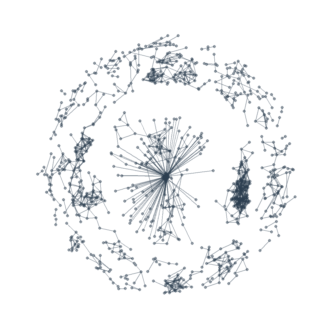

Nodes and Edges

Graph Manipulation

customer_tbl_graph <- customer_correlation_matrix %>%
    prep_corr_matrix_for_tbl_graph(edge_limit = 0.997) %>%
    as_tbl_graph(directed = FALSE)

customer_tbl_graph

## # A tbl_graph: 890 nodes and 1502 edges
## #
## # An undirected simple graph with 213 components
## #
## # Node Data: 890 x 1 (active)
##   name  
##   <chr> 
## 1 C16180
## 2 C17657
## 3 C14958
## 4 C11181
## 5 C12206
## 6 C13649
## # ... with 884 more rows
## #
## # Edge Data: 1,502 x 3
##    from    to weight
##   <int> <int>  <dbl>
## 1     1   543  0.997
## 2     2   543  0.998
## 3     3   544  0.999
## # ... with 1,499 more rows

Ranking Nodes - Rank by topological traits (Find out which customers are the most important vs the other customers)

customer_tbl_graph %>%
    activate(nodes) %>%
    mutate(node_rank = node_rank_traveller()) %>%
    arrange(node_rank)

## # A tbl_graph: 890 nodes and 1502 edges
## #
## # An undirected simple graph with 213 components
## #
## # Node Data: 890 x 2 (active)
##   name   node_rank
##   <chr>      <int>
## 1 C14001         1
## 2 C10045         2
## 3 C16928         3
## 4 C18807         4
## 5 C16688         5
## 6 C13730         6
## # ... with 884 more rows
## #
## # Edge Data: 1,502 x 3
##    from    to weight
##   <int> <int>  <dbl>
## 1   681   682  0.997
## 2   680   681  0.998
## 3   357   358  0.999
## # ... with 1,499 more rows

Centrality - Number of edges going in/out of node (The node with highest number of edges is the most important)

customer_tbl_graph %>%
    activate(nodes) %>%
    mutate(neighbors = centrality_degree()) %>%
    arrange(desc(neighbors))

## # A tbl_graph: 890 nodes and 1502 edges
## #
## # An undirected simple graph with 213 components
## #
## # Node Data: 890 x 2 (active)
##   name   neighbors
##   <chr>      <dbl>
## 1 C18341        37
## 2 C18363        26
## 3 C18811        25
## 4 C18913        25
## 5 C18271        24
## 6 C16626        23
## # ... with 884 more rows
## #
## # Edge Data: 1,502 x 3
##    from    to weight
##   <int> <int>  <dbl>
## 1   241   402  0.997
## 2   242   402  0.998
## 3   470   688  0.999
## # ... with 1,499 more rows

Grouping Nodes (Clustering)

grouped_tbl_graph <- customer_tbl_graph %>%
    activate(nodes) %>%
    mutate(neighbors = centrality_degree()) %>%
    
    mutate(group = group_components()) %>%
    
    arrange(desc(neighbors)) %>%
    mutate(group_lump = group %>% as_factor() %>% fct_lump(n = 5))

grouped_tbl_graph %>%
    ggraph(layout = "kk") +
    geom_edge_link(alpha = 0.5) +
    geom_node_point(aes(color = group_lump), alpha = 0.5, size = 3) +
    
    theme_graph() +
    scale_color_tq(theme = "light") +
    theme(legend.position = "bottom") +
    labs(title = "Customer Network Detection")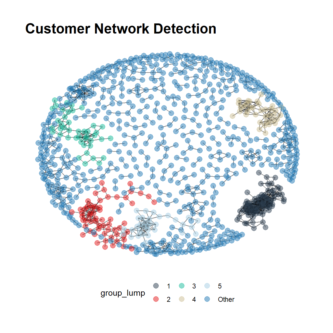

Community Analysis

Join Communities and Inspect Key Features

credit_card_group_tbl <- credit_card_tbl %>%
    left_join(as_tibble(grouped_tbl_graph), by = c("CUST_ID" = "name")) %>%
    select(group_lump, CUST_ID, everything()) %>%
    filter(!is.na(group_lump))

credit_card_group_tbl %>% glimpse()

## Rows: 890
## Columns: 21
## $ group_lump                       <fct> Other, Other, Other, 2, 2, 1, Othe...
## $ CUST_ID                          <chr> "C10005", "C10011", "C10015", "C10...
## $ BALANCE                          <dbl> 817.714335, 1293.124939, 2772.7727...
## $ BALANCE_FREQUENCY                <dbl> 1.000000, 1.000000, 1.000000, 1.00...
## $ PURCHASES                        <dbl> 16.00, 920.12, 0.00, 399.60, 233.2...
## $ ONEOFF_PURCHASES                 <dbl> 16.00, 0.00, 0.00, 0.00, 0.00, 0.0...
## $ INSTALLMENTS_PURCHASES           <dbl> 0.00, 920.12, 0.00, 399.60, 233.28...
## $ CASH_ADVANCE                     <dbl> 0.00000, 0.00000, 346.81139, 0.000...
## $ PURCHASES_FREQUENCY              <dbl> 0.083333, 1.000000, 0.000000, 1.00...
## $ ONEOFF_PURCHASES_FREQUENCY       <dbl> 0.083333, 0.000000, 0.000000, 0.00...
## $ PURCHASES_INSTALLMENTS_FREQUENCY <dbl> 0.000000, 1.000000, 0.000000, 1.00...
## $ CASH_ADVANCE_FREQUENCY           <dbl> 0.000000, 0.000000, 0.083333, 0.00...
## $ CASH_ADVANCE_TRX                 <dbl> 0, 0, 1, 0, 0, 1, 1, 0, 1, 1, 0, 4...
## $ PURCHASES_TRX                    <dbl> 1, 12, 0, 12, 12, 0, 0, 1, 0, 0, 3...
## $ CREDIT_LIMIT                     <dbl> 1200, 1200, 3000, 3000, 1000, 1800...
## $ PAYMENTS                         <dbl> 678.33476, 1083.30101, 805.64797, ...
## $ MINIMUM_PAYMENTS                 <dbl> 244.79124, 2172.69776, 989.96287, ...
## $ PRC_FULL_PAYMENT                 <dbl> 0.000000, 0.000000, 0.000000, 0.00...
## $ TENURE                           <dbl> 12, 12, 12, 12, 12, 12, 12, 12, 8,...
## $ neighbors                        <dbl> 2, 1, 5, 3, 17, 15, 1, 2, 1, 2, 1,...
## $ group                            <int> 9, 84, 12, 2, 2, 1, 85, 6, 86, 41,...

plot_density_by <- function(data, col, group_focus = 1, ncol = 1) {
    
    col_expr <- enquo(col)
    
    data %>%
        mutate(focus = as.character(group_lump)) %>%
        select(focus, everything()) %>%
        mutate(focus = ifelse(as.character(focus) == as.character(group_focus), 
                                    "1", "Other")) %>%
        mutate(focus = as.factor(focus)) %>%
        
        ggplot(aes(!! col_expr, fill = focus)) +
        geom_density(alpha = 0.4) +
        facet_wrap(~ focus, ncol = ncol) +
        scale_fill_tq() +
        theme_tq()
}

Group 1.

By Balance

For this first group we can see that every customers has bimodal and trimodal relationships but you can see that for group 1 everyone has pretty high balance compare to the spike vs the other. This categorizes the group 1 as they tend to have a higher balance.

credit_card_group_tbl %>% plot_density_by(BALANCE, group_focus = 1)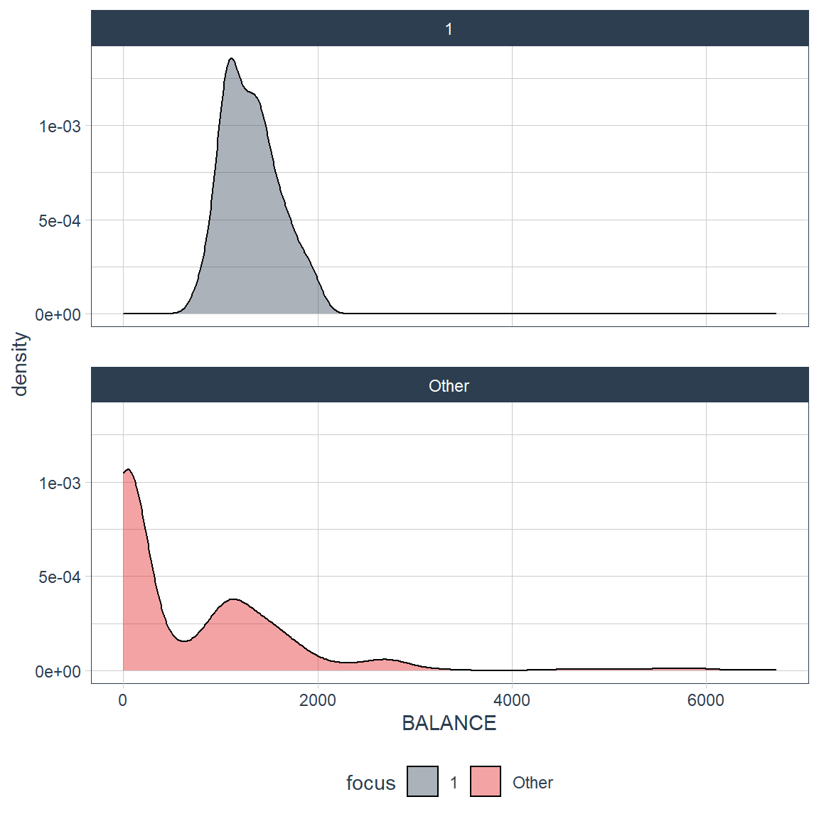

By Min Payment

credit_card_group_tbl %>% plot_density_by(MINIMUM_PAYMENTS, group_focus = 1)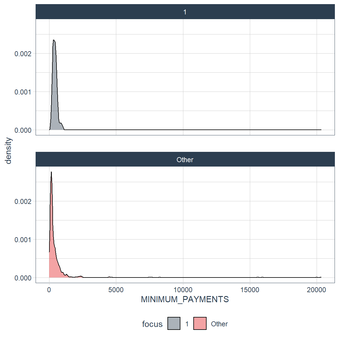

credit_card_group_tbl %>% plot_density_by(log(MINIMUM_PAYMENTS), group_focus = 1)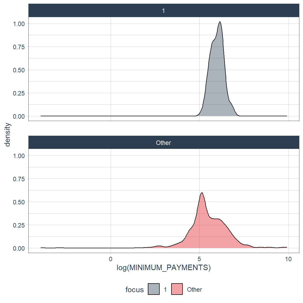

Cash Advance Frequency

credit_card_group_tbl %>% plot_density_by(CASH_ADVANCE_FREQUENCY, group_focus = 1)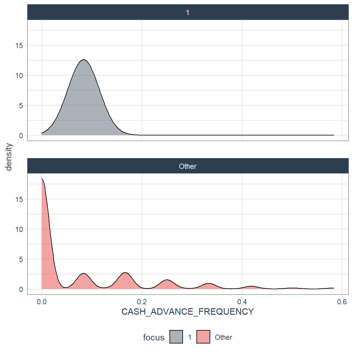

Group 2

By Balance

credit_card_group_tbl %>% plot_density_by(BALANCE, group_focus = 2, ncol = 1)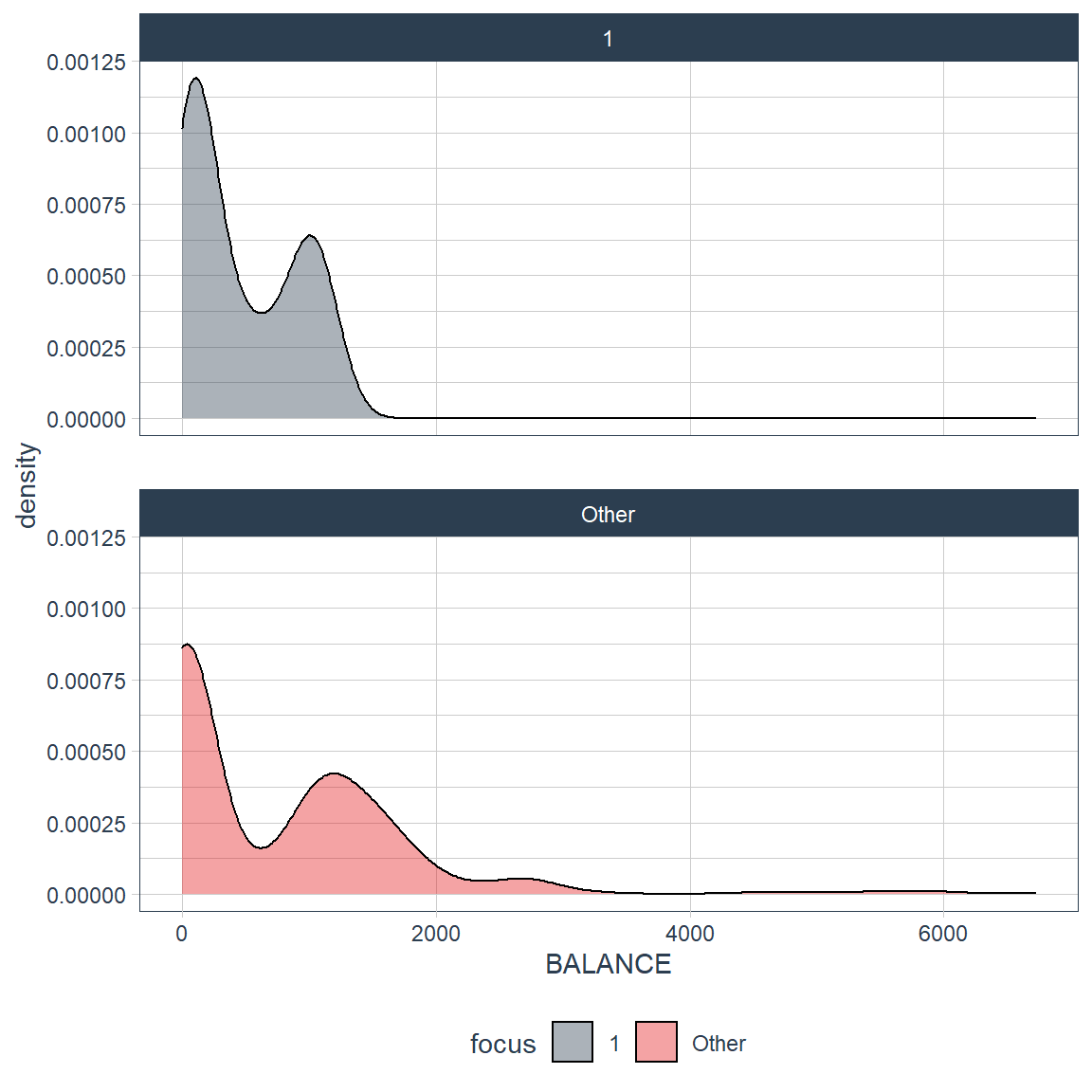

credit_card_group_tbl %>% plot_density_by(log(BALANCE), group_focus = 2, ncol = 1)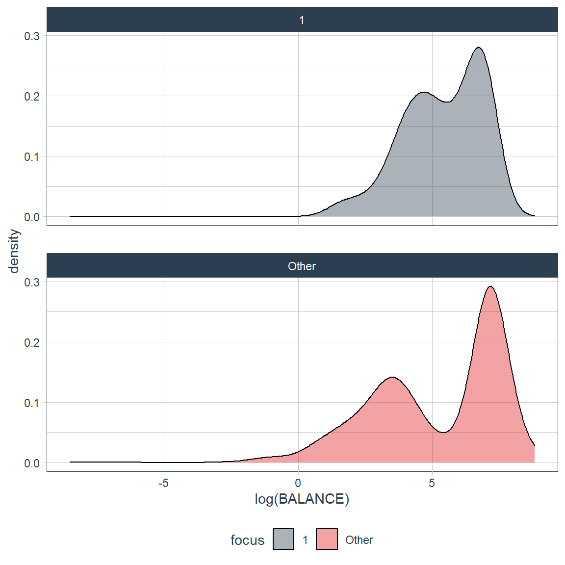

By Min Payment

credit_card_group_tbl %>% plot_density_by(MINIMUM_PAYMENTS, group_focus = 2)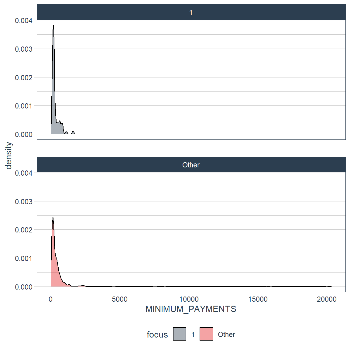

credit_card_group_tbl %>% plot_density_by(log(MINIMUM_PAYMENTS), group_focus = 2)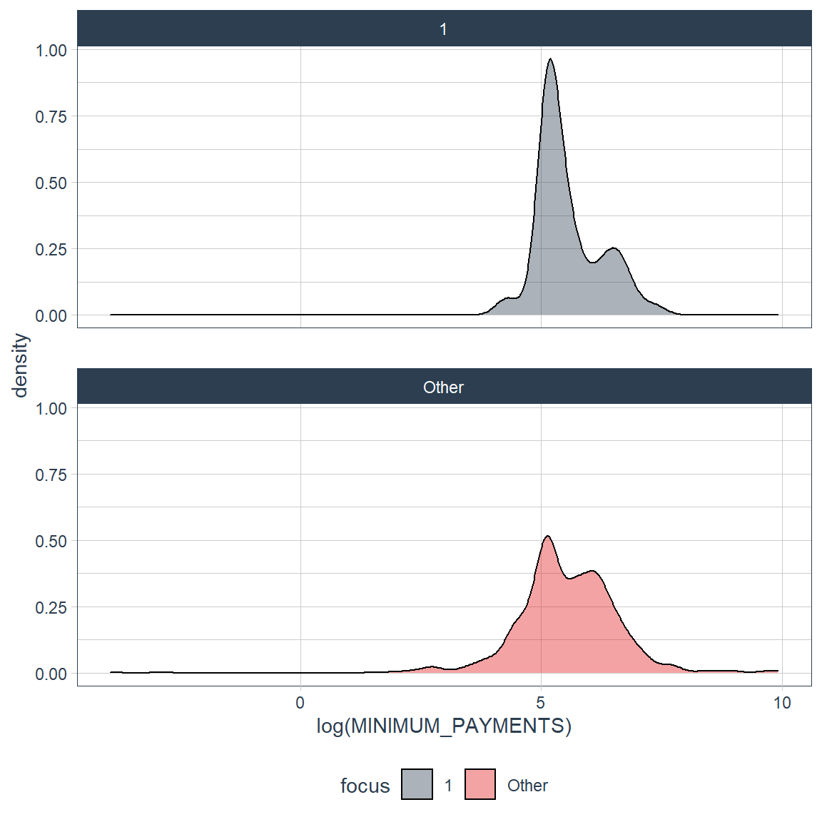

Cash Advance Frequency

credit_card_group_tbl %>% plot_density_by(CASH_ADVANCE_FREQUENCY, group_focus = 2)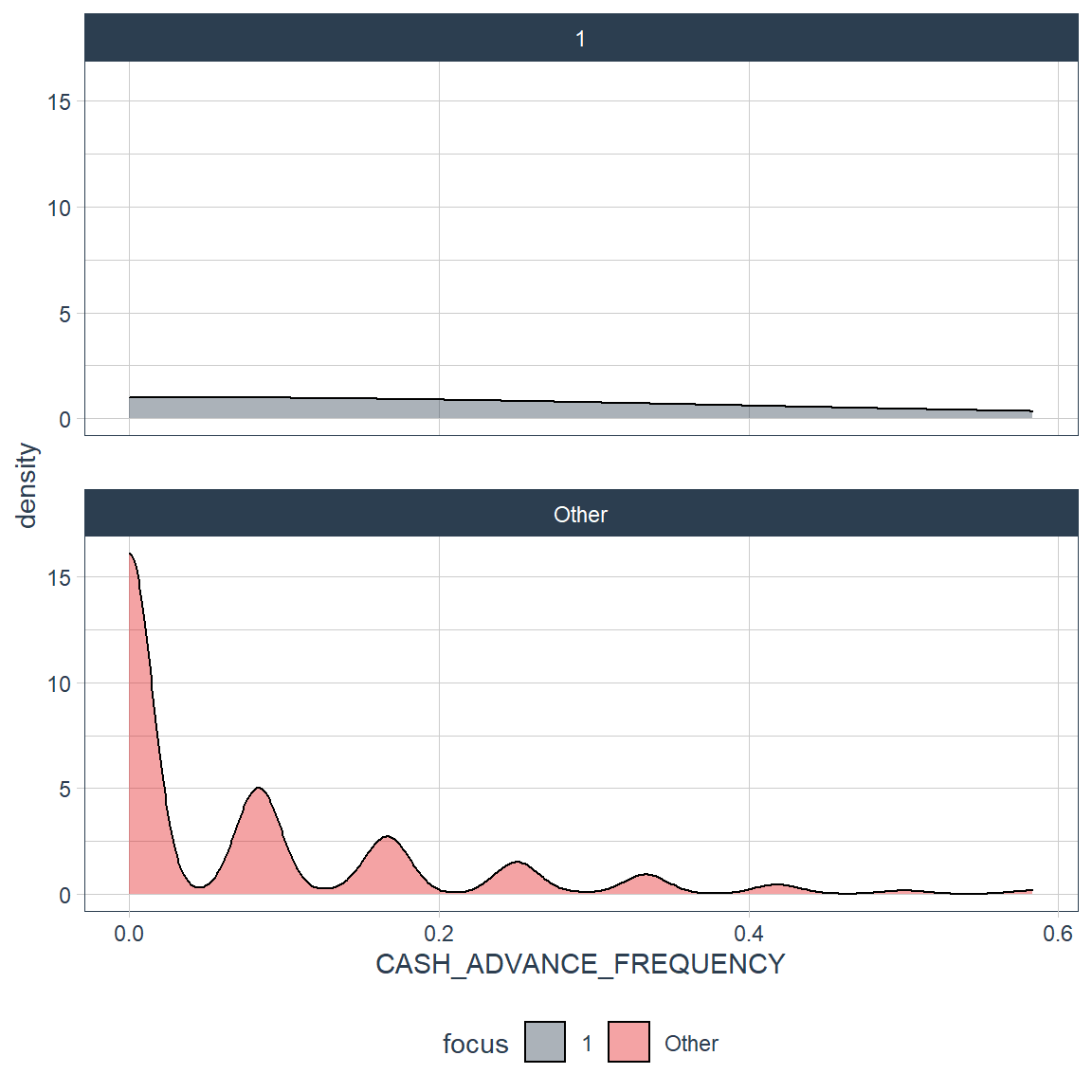

H2O and LIME

Predict and Explain Customer Segments.

H2O -Multi-class prediction with H2O AutoML -Training a model to detect which group each customer belongs to which group. LIME Explanation -ML Explanation of which features contribute to each class with LIME -Returns a function called explain_customer()

source("h2o_lime.R")

## 
## H2O is not running yet, starting it now...
## 
## Note:  In case of errors look at the following log files:
##     C:\Users\Apple\AppData\Local\Temp\RtmpyKhEA7\filea7c74154fc9/h2o_Apple_started_from_r.out
##     C:\Users\Apple\AppData\Local\Temp\RtmpyKhEA7\filea7c36525d49/h2o_Apple_started_from_r.err
## 
## 
## Starting H2O JVM and connecting: ... Connection successful!
## 
## R is connected to the H2O cluster: 
##     H2O cluster uptime:         19 seconds 271 milliseconds 
##     H2O cluster timezone:       Asia/Singapore 
##     H2O data parsing timezone:  UTC 
##     H2O cluster version:        3.30.1.3 
##     H2O cluster version age:    5 months and 15 days !!! 
##     H2O cluster name:           H2O_started_from_R_Apple_rqh772 
##     H2O cluster total nodes:    1 
##     H2O cluster total memory:   1.96 GB 
##     H2O cluster total cores:    4 
##     H2O cluster allowed cores:  4 
##     H2O cluster healthy:        TRUE 
##     H2O Connection ip:          localhost 
##     H2O Connection port:        54321 
##     H2O Connection proxy:       NA 
##     H2O Internal Security:      FALSE 
##     H2O API Extensions:         Amazon S3, Algos, AutoML, Core V3, TargetEncoder, Core V4 
##     R Version:                  R version 4.0.2 (2020-06-22) 
## 
## 
  |                                                                            
  |                                                                      |   0%
  |                                                                            
  |======================================================================| 100%
## 
  |                                                                            
  |                                                                      |   0%
  |                                                                            
  |=                                                                     |   1%
  |                                                                            
  |==================================================================    |  95%
  |                                                                            
  |======================================================================| 100%

credit_card_group_tbl

## # A tibble: 890 x 21
##    group_lump CUST_ID BALANCE BALANCE_FREQUEN~ PURCHASES ONEOFF_PURCHASES
##    <fct>      <chr>     <dbl>            <dbl>     <dbl>            <dbl>
##  1 Other      C10005     818.            1          16               16  
##  2 Other      C10011    1293.            1         920.               0  
##  3 Other      C10015    2773.            1           0                0  
##  4 2          C10026     170.            1         400.               0  
##  5 2          C10028     126.            1         233.               0  
##  6 1          C10036    1656.            1           0                0  
##  7 Other      C10045    1361.            1           0                0  
##  8 Other      C10063    1556.            1          66.2             66.2
##  9 Other      C10069     810.            0.875       0                0  
## 10 Other      C10082    1206.            1           0                0  
## # ... with 880 more rows, and 15 more variables: INSTALLMENTS_PURCHASES <dbl>,
## #   CASH_ADVANCE <dbl>, PURCHASES_FREQUENCY <dbl>,
## #   ONEOFF_PURCHASES_FREQUENCY <dbl>, PURCHASES_INSTALLMENTS_FREQUENCY <dbl>,
## #   CASH_ADVANCE_FREQUENCY <dbl>, CASH_ADVANCE_TRX <dbl>, PURCHASES_TRX <dbl>,
## #   CREDIT_LIMIT <dbl>, PAYMENTS <dbl>, MINIMUM_PAYMENTS <dbl>,
## #   PRC_FULL_PAYMENT <dbl>, TENURE <dbl>, neighbors <dbl>, group <int>

h2o.predict(h2o_model, newdata = as.h2o(credit_card_group_tbl)) %>%
  as_tibble()

## 
  |                                                                            
  |                                                                      |   0%
  |                                                                            
  |======================================================================| 100%
## 
  |                                                                            
  |                                                                      |   0%
  |                                                                            
  |======================================================================| 100%

## # A tibble: 890 x 7
##    predict     p1        p2        p3    p4       p5   Other
##    <fct>    <dbl>     <dbl>     <dbl> <dbl>    <dbl>   <dbl>
##  1 Other   0      0.000101  0.0000782     0 0.000428 0.999  
##  2 Other   0      0         0.0000782     0 0        1.00   
##  3 Other   0.0226 0.0000985 0.0000764     0 0.000419 0.977  
##  4 2       0      0.944     0.0000782     0 0        0.0556 
##  5 2       0      1.00      0.0000782     0 0.000262 0      
##  6 1       0.998  0.000102  0.0000788     0 0.000432 0.00124
##  7 Other   0.0999 0.0000907 0.0000704     0 0.000385 0.900  
##  8 Other   0      0.000101  0             0 0.000428 0.999  
##  9 Other   0.0526 0.0000955 0.0000741     0 0.000406 0.947  
## 10 Other   0.136  0.0000871 0.0000676     0 0.000370 0.864  
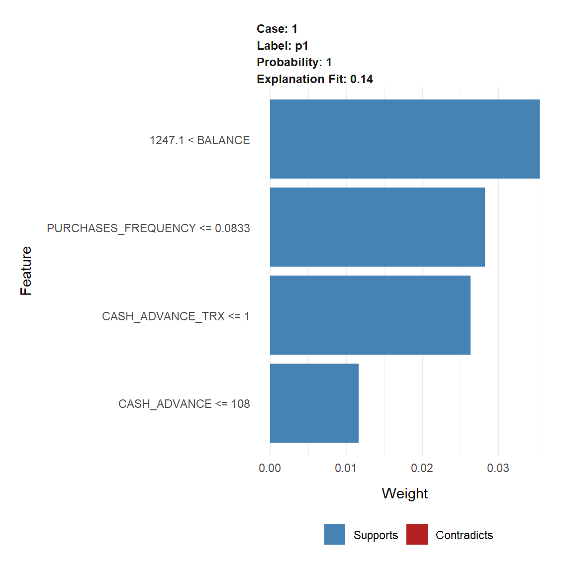
## # ... with 880 more rows

Explain why customers 6 belong to communities.

explain_customer(6)

## 
  |                                                                            
  |                                                                      |   0%
  |                                                                            
  |======================================================================| 100%
## 
  |                                                                            
  |                                                                      |   0%
  |                                                                            
  |======================================================================| 100%