Product Analytics
# Load libraries ----

# Work horse packages
library(tidyverse)
library(lubridate)

# theme_tq()
library(tidyquant)

# Excel Files
library(readxl)
library(writexl)

# Visualization
library(plotly)

# Preprocessing and Sampling
library(recipes)
library(rsample)

# Model Error Metrics
library(yardstick)

  # Modeling
library(parsnip)
library(glmnet)
library(randomForest)
library(xgboost)

# Plot Decision Trees
library(rpart)
library(rpart.plot)
library(ggrepel)

library(ranger)
library(kernlab)


library(broom)
library(uwot)

# Importing Files ----
bikes_tbl <- read_excel(path = "00_data/bike_sales/data_raw/bikes.xlsx")
bikeshops_tbl <- read_excel(path = "00_data/bike_sales/data_raw/bikeshops.xlsx")
orderlines_tbl <- read_excel(path = "00_data/bike_sales/data_raw/orderlines.xlsx")

source("00_scripts/plot_sales.R")
source("00_scripts/plot_customer_segmentation.R")
Examining Data
Bike Datasets
glimpse(bikes_tbl)## Rows: 97
## Columns: 4
## $ bike.id <dbl> 1, 2, 3, 4, 5, 6, 7, 8, 9, 10, 11, 12, 13, 14, 15, 16, ...
## $ model <chr> "Supersix Evo Black Inc.", "Supersix Evo Hi-Mod Team", ...
## $ description <chr> "Road - Elite Road - Carbon", "Road - Elite Road - Carb...
## $ price <dbl> 12790, 10660, 7990, 5330, 4260, 3940, 3200, 2660, 2240,...bikes_tbl## # A tibble: 97 x 4
## bike.id model description price
## <dbl> <chr> <chr> <dbl>
## 1 1 Supersix Evo Black Inc. Road - Elite Road - Carbon 12790
## 2 2 Supersix Evo Hi-Mod Team Road - Elite Road - Carbon 10660
## 3 3 Supersix Evo Hi-Mod Dura Ace 1 Road - Elite Road - Carbon 7990
## 4 4 Supersix Evo Hi-Mod Dura Ace 2 Road - Elite Road - Carbon 5330
## 5 5 Supersix Evo Hi-Mod Utegra Road - Elite Road - Carbon 4260
## 6 6 Supersix Evo Red Road - Elite Road - Carbon 3940
## 7 7 Supersix Evo Ultegra 3 Road - Elite Road - Carbon 3200
## 8 8 Supersix Evo Ultegra 4 Road - Elite Road - Carbon 2660
## 9 9 Supersix Evo 105 Road - Elite Road - Carbon 2240
## 10 10 Supersix Evo Tiagra Road - Elite Road - Carbon 1840
## # ... with 87 more rowsBike Shops
glimpse(bikeshops_tbl)## Rows: 30
## Columns: 3
## $ bikeshop.id <dbl> 1, 2, 3, 4, 5, 6, 7, 8, 9, 10, 11, 12, 13, 14, 15, 16...
## $ bikeshop.name <chr> "Pittsburgh Mountain Machines", "Ithaca Mountain Clim...
## $ location <chr> "Pittsburgh, PA", "Ithaca, NY", "Columbus, OH", "Detr...bikeshops_tbl## # A tibble: 30 x 3
## bikeshop.id bikeshop.name location
## <dbl> <chr> <chr>
## 1 1 Pittsburgh Mountain Machines Pittsburgh, PA
## 2 2 Ithaca Mountain Climbers Ithaca, NY
## 3 3 Columbus Race Equipment Columbus, OH
## 4 4 Detroit Cycles Detroit, MI
## 5 5 Cincinnati Speed Cincinnati, OH
## 6 6 Louisville Race Equipment Louisville, KY
## 7 7 Nashville Cruisers Nashville, TN
## 8 8 Denver Bike Shop Denver, CO
## 9 9 Minneapolis Bike Shop Minneapolis, MN
## 10 10 Kansas City 29ers Kansas City, KS
## # ... with 20 more rowsBike Orders
glimpse(orderlines_tbl)## Rows: 15,644
## Columns: 7
## $ ...1 <chr> "1", "2", "3", "4", "5", "6", "7", "8", "9", "10", "11"...
## $ order.id <dbl> 1, 1, 2, 2, 3, 3, 3, 3, 3, 4, 5, 5, 5, 5, 6, 6, 6, 6, 7...
## $ order.line <dbl> 1, 2, 1, 2, 1, 2, 3, 4, 5, 1, 1, 2, 3, 4, 1, 2, 3, 4, 1...
## $ order.date <dttm> 2015-01-07, 2015-01-07, 2015-01-10, 2015-01-10, 2015-0...
## $ customer.id <dbl> 2, 2, 10, 10, 6, 6, 6, 6, 6, 22, 8, 8, 8, 8, 16, 16, 16...
## $ product.id <dbl> 48, 52, 76, 52, 2, 50, 1, 4, 34, 26, 96, 66, 35, 72, 45...
## $ quantity <dbl> 1, 1, 1, 1, 1, 1, 1, 1, 1, 1, 1, 2, 1, 1, 1, 1, 1, 1, 1...orderlines_tbl## # A tibble: 15,644 x 7
## ...1 order.id order.line order.date customer.id product.id quantity
## <chr> <dbl> <dbl> <dttm> <dbl> <dbl> <dbl>
## 1 1 1 1 2015-01-07 00:00:00 2 48 1
## 2 2 1 2 2015-01-07 00:00:00 2 52 1
## 3 3 2 1 2015-01-10 00:00:00 10 76 1
## 4 4 2 2 2015-01-10 00:00:00 10 52 1
## 5 5 3 1 2015-01-10 00:00:00 6 2 1
## 6 6 3 2 2015-01-10 00:00:00 6 50 1
## 7 7 3 3 2015-01-10 00:00:00 6 1 1
## 8 8 3 4 2015-01-10 00:00:00 6 4 1
## 9 9 3 5 2015-01-10 00:00:00 6 34 1
## 10 10 4 1 2015-01-11 00:00:00 22 26 1
## # ... with 15,634 more rowsData Wrangling
bike_orderlines_joined_tbl <- orderlines_tbl %>%
    left_join(bikes_tbl, by = c("product.id" = "bike.id")) %>%
    left_join(bikeshops_tbl, by = c("customer.id" = "bikeshop.id"))


bike_orderlines_tbl <- bike_orderlines_joined_tbl %>%
    separate(
        description,
        into = c("category_1", "category_2", "frame_material"),
        sep = " - "
    ) %>%
    separate(location,
             into = c("city", "state"),
             sep = ", ") %>%
    mutate(total_price = quantity * price) %>%
    select(-...1,-ends_with(".id")) %>%
    bind_cols(bike_orderlines_joined_tbl %>%
                  select(order.id)) %>%
    select(
        contains("date"),
        contains("id"),
        contains("order"),
        quantity,
        price,
        total_price,
        everything()
    ) %>%
    set_names(names(.) %>% str_replace_all("\\.", "_"))

sales_by_year_category_2_tbl <- bike_orderlines_tbl %>%
    select(order_date, category_2, total_price) %>%

    mutate(order_date = ymd(order_date)) %>%
    mutate(year = year(order_date)) %>%

    group_by(category_2, year) %>%
    summarize(revenue = sum(total_price)) %>%
    ungroup() %>%

    mutate(category_2 = fct_reorder2(category_2, year, revenue))
Business Insights
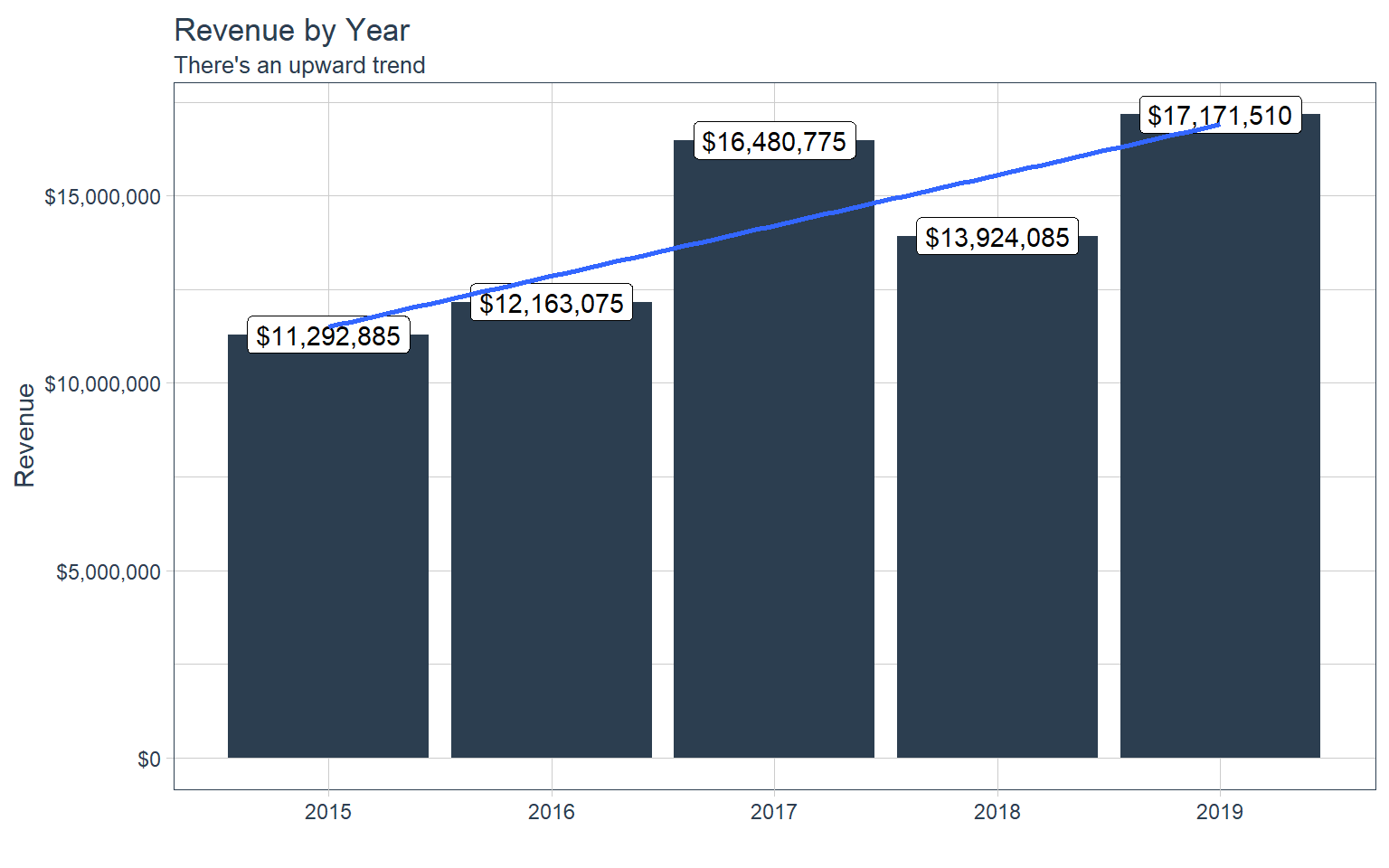
Sales
# Step 1 - Manipulate
sales_by_year_tbl <- bike_orderlines_tbl %>%
    # Get columns we want
    select(order_date, total_price) %>%
    mutate(year = year(order_date)) %>%
    # groupings
    group_by(year) %>%
    summarize(sales = sum(total_price)) %>%
    ungroup() %>%
    # get dollar text
    mutate(sales_text = scales::dollar(sales))

# Step 2 - Visualize
sales_by_year_tbl %>%
    ggplot(aes(x = year, y = sales)) +
    geom_col(fill = "#2C3E50") +
    geom_label(aes(label = sales_text)) +
    geom_smooth(method = "lm",
                se = FALSE) +
    theme_tq() +
    scale_y_continuous(labels = scales::dollar) +
    labs(
        title = "Revenue by Year",
        subtitle = "There's an upward trend",
        x = "",
        y = "Revenue"
    )
revenue_by_year_tbl <- bike_orderlines_tbl %>%
    select(order_date, total_price) %>%
    mutate(year = year(order_date)) %>%

    group_by(year) %>%
    summarize(revenue = sum(total_price)) %>%
    ungroup()
revenue_by_year_tbl %>%

# Canvas
ggplot(aes(x = year, y = revenue, color = revenue)) +
  # Geometries
  geom_line(size = 1) +
  geom_point(size = 5) +
  geom_smooth(method = "lm", se = FALSE) +
  # Formatting
  expand_limits(y = 0) +
  scale_color_continuous(low = "red", high = "black",labels = scales::dollar_format(scale = 1/1e6, suffix = "M")) +
  scale_y_continuous(labels = scales::dollar_format(scale = 1/1e6, suffix = "M")) +
  labs(
    title = "Revenue",
    subtitle = "Sales are trending up and to the right!",
    x = "",
    y = "Sales (Millions)",
    color = "Rev ($M)",
    caption = "What's happening?\nSales numbers showing year-over-year growth.") +
    theme_bw() +
    theme(legend.position = "right", legend.direction = "vertical")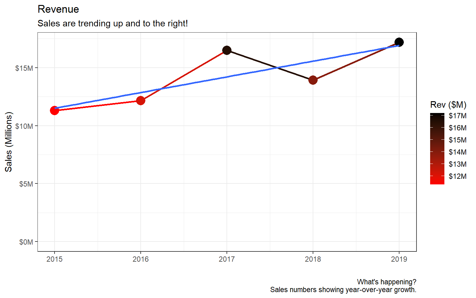
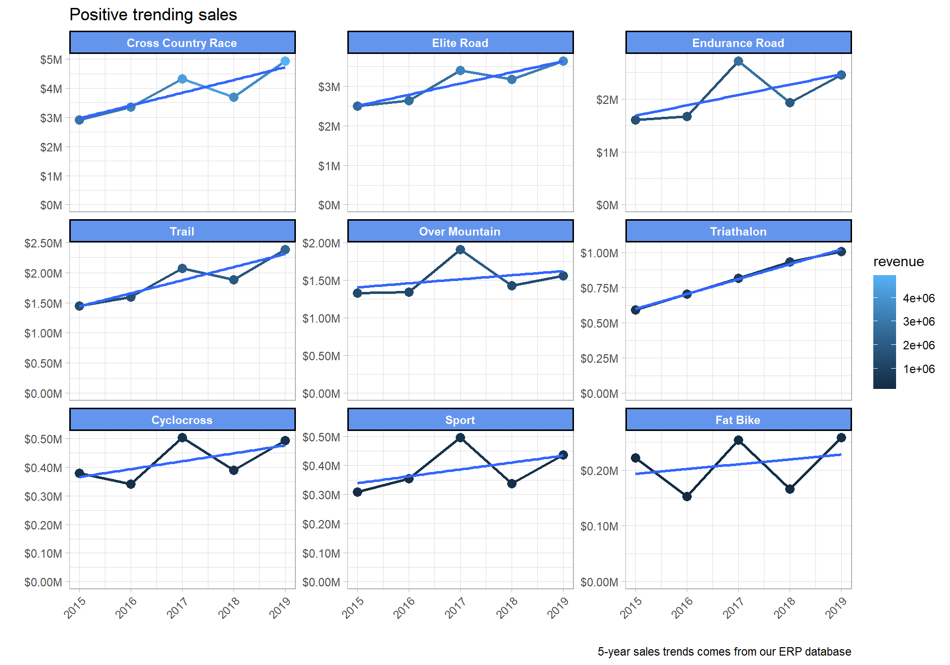
sales_by_year_category_2_tbl %>%
  ggplot(mapping = aes(x = year, y = revenue, color = revenue)) +
  geom_line(size = 1) +
  geom_point(size = 3) +
  facet_wrap(~ category_2, scales = "free_y") +
  expand_limits(y = 0) +
  scale_y_continuous(labels = scales::dollar_format(scale = 1e-6, suffix = "M")) +
  geom_smooth(method = "lm", se = FALSE) +
  theme_light() +
  theme(axis.text.x = element_text(angle   = 45, hjust = 1),
        strip.background = element_rect(
          color  = "black",
          fill = "cornflowerblue",
          size = 1),
        strip.text = element_text(face = "bold", color = "white")) +
  labs(
        title = "Positive trending sales",
        caption = "5-year sales trends comes from our ERP database",
        x = "",
        y = ""
    )
Monthly Revenue
Describe revenue by Month, expose cyclic nature.
# Data Manipulation
revenue_by_month_tbl <- bike_orderlines_tbl %>%
  select(order_date, total_price) %>%
  mutate(year_month = floor_date(order_date, "months") %>% ymd()) %>%
  group_by(year_month) %>%
  summarize(revenue = sum(total_price)) %>%
  ungroup()

# Line Plot
revenue_by_month_tbl %>%
  ggplot(
    mapping = aes(x = year_month, y = revenue)) +
  geom_line() +
  geom_smooth(span = 0.2) +
  theme_classic()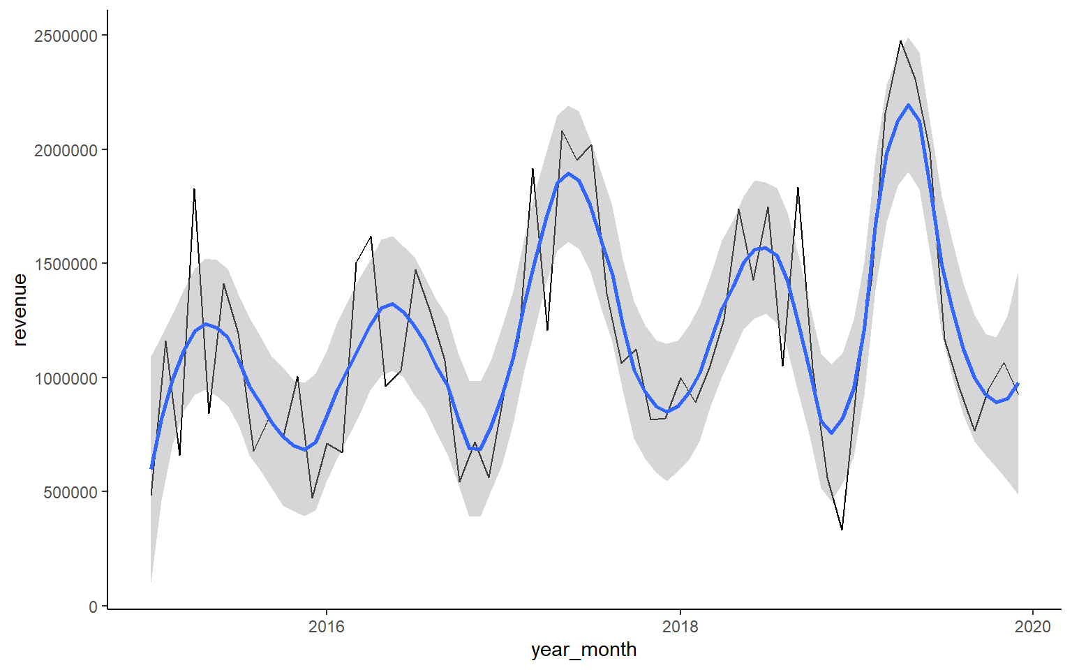
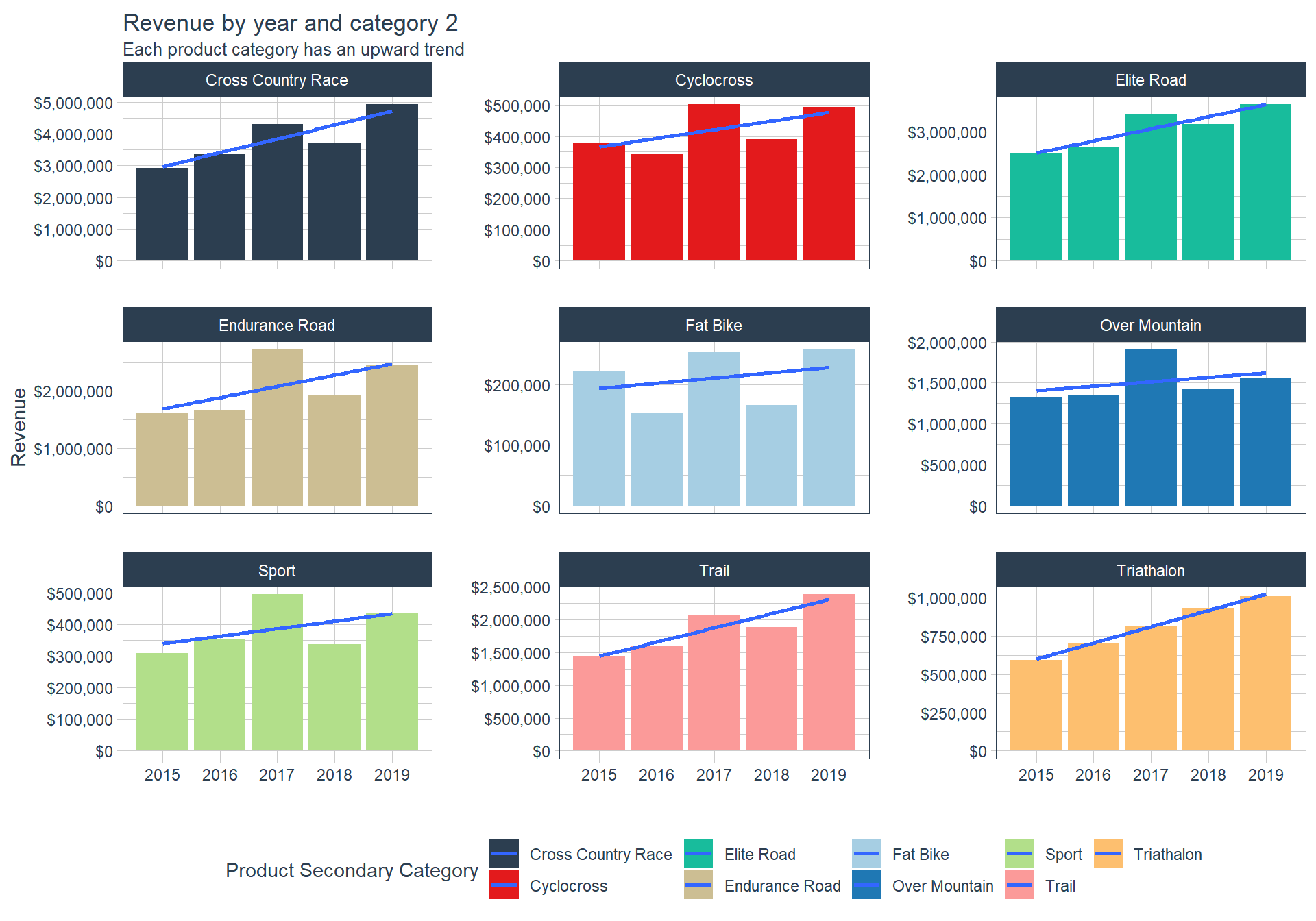
Annual sales by secondary category
# Step 1 - Manipulate
sales_by_year_cat_2_tbl <- bike_orderlines_tbl %>%
    select(order_date, category_2, total_price) %>%
    mutate(year = year(order_date)) %>%
    group_by(year, category_2) %>%
    summarize(sales = sum(total_price)) %>%
    ungroup() %>%
    mutate(sales_text = scales::dollar(sales))

# Step 2 - Visualize
sales_by_year_cat_2_tbl %>%
    ggplot(aes(x = year, y = sales, fill = category_2)) +
    geom_col() +
    geom_smooth(method = "lm",
                se = FALSE) +
    facet_wrap(~ category_2, scales = "free_y") +
    theme_tq() +
    scale_fill_tq() +
    scale_y_continuous(labels = scales::dollar) +
    labs(
        title = "Revenue by year and category 2",
        subtitle = "Each product category has an upward trend",
        x = "",
        y = "Revenue",
        fill = "Product Secondary Category"
    )
# - Great way to tease out variation by category
sales_by_year_category_2_tbl %>%
  ggplot(mapping = aes(x = year, y = revenue, color = category_2)) +
  geom_line(size = 1, color = "black") +
  geom_point() +
  geom_smooth(method = "lm", se = F) +
  facet_wrap(~ category_2, scales = "free_y") +
  scale_y_continuous(
    labels = scales::dollar_format(scale = 1/1e6, suffix = "M")) +
  expand_limits(y = 0) +
  labs(title = "Sales by Category 2", color = "Category 2", x = "", y = "Revenue") +
  theme_light() +
  theme(axis.text.x = element_text(angle   = 45, hjust = 1),
        strip.background = element_rect(
          color  = "black",
          fill = "cornflowerblue",
          size = 1),
        strip.text = element_text(face = "bold", color = "white"))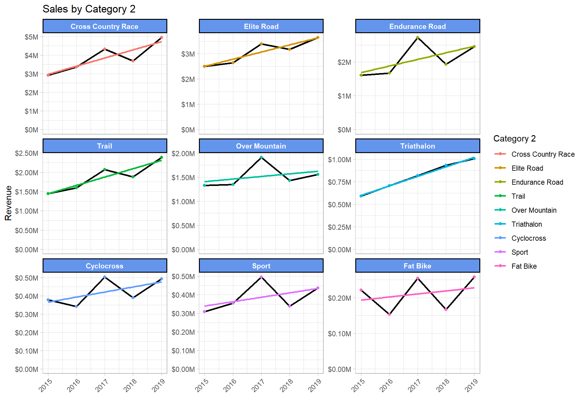
Total revenue by category
# Bar / Column Plots ---- Categories

revenue_by_category_tbl <- bike_orderlines_tbl %>%
  select(category_2, category_1, total_price) %>%

  group_by(category_2, category_1) %>%
  summarise(total_revenue = sum(total_price)) %>%
  ungroup() %>%

  arrange(desc(total_revenue)) %>%
  mutate(category_2 = as_factor(category_2) %>% fct_rev())

# Bar Plot
g <- revenue_by_category_tbl %>%
  ggplot(aes(category_2, total_revenue, fill = category_1)) +

  # Geoms
  geom_col() +
  coord_flip() +

  # Formatting
  scale_fill_tq() +
  scale_y_continuous(labels = scales::dollar_format(scale = 1e-6, suffix = "M")) +
  theme_tq() +
  labs(
    title = "Total Revenue by Category",
    x = "", y = "", fill = ""
  )

ggplotly(g)
# Fill -----
# - Used with fill of rectangular objects.
sales_by_year_category_2_tbl %>%
ggplot(mapping = aes(x = year, y = revenue, fill = category_2)) +
geom_col() +
scale_y_continuous(labels = scales::dollar_format(scale = 1/1e6, suffix = "M"))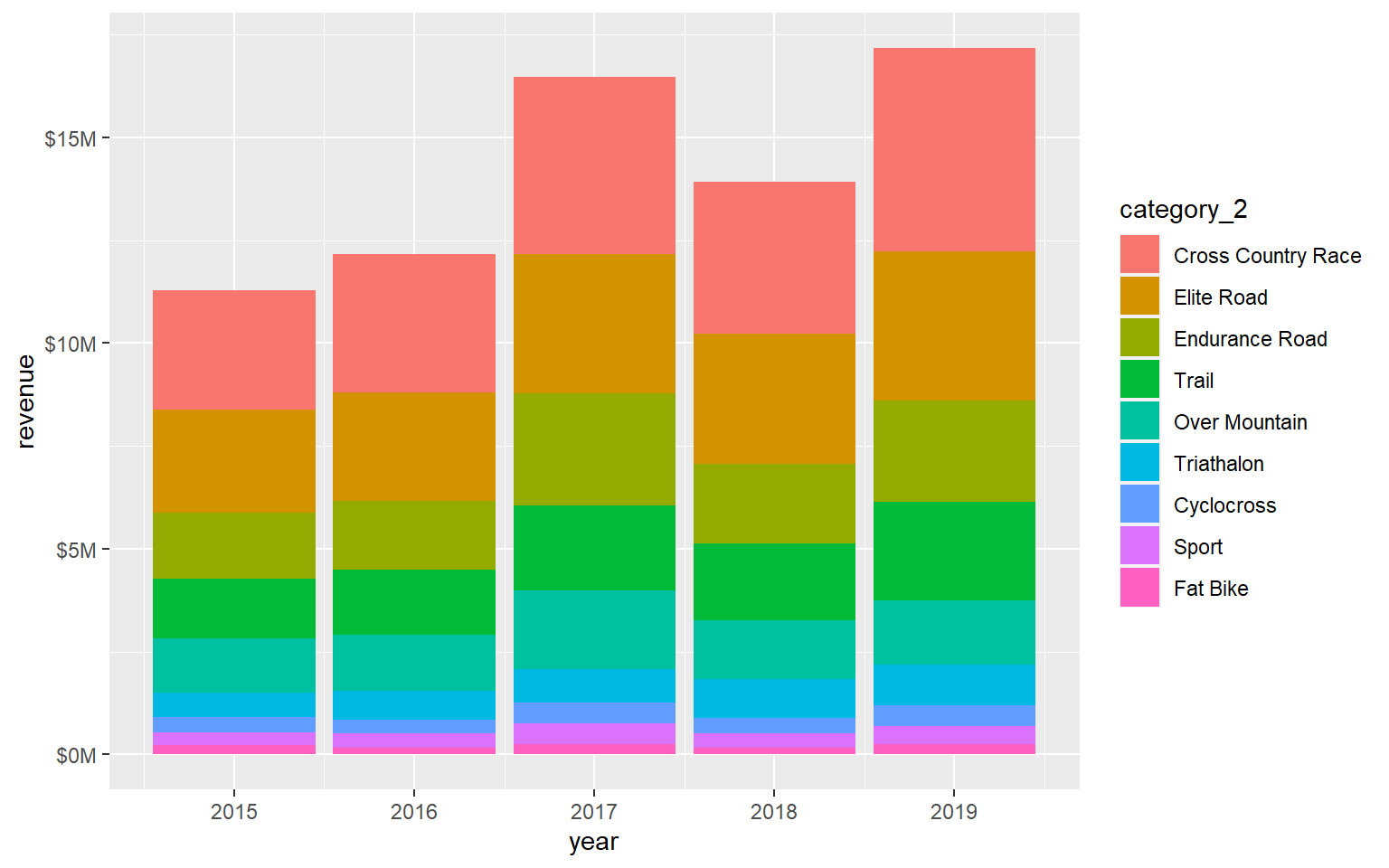
# Stacked Area
sales_by_year_category_2_tbl %>%
  ggplot(mapping = aes(x = year, y = revenue, fill = category_2)) +
  geom_area(color = "black") +
  scale_fill_brewer(palette = "Blues", direction = -1) +
  scale_y_continuous(labels = scales::dollar_format(scale = 1e-6, suffix = "M")) +
  labs(
    title = "Sales over year by secondary category",
    subtitle = "Sales trending upward",
    caption = "Data comes from our ERP database",
    x = "",
    y = "Revenue ($M)",
    fill = "Category 2") +
  theme_light() +
  theme(
    title = element_text(face = "bold", color = "#08306B"))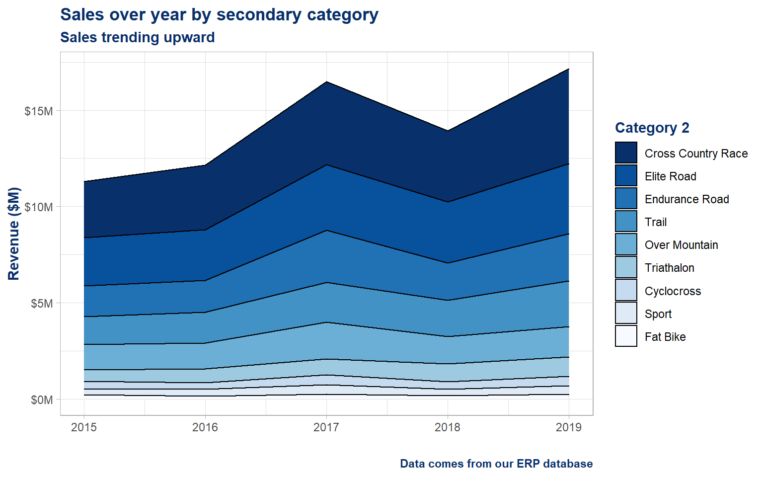
Prices
Inspecting the distribution of a variable
# Histogram / Density Plots
# Inspecting the distribution of a variable

bike_orderlines_tbl %>%
  distinct(model, price) %>%
  ggplot(mapping = aes(x = price)) +
  geom_histogram(bins = 25, fill = "blue", color = "white") +
  tidyquant::theme_tq()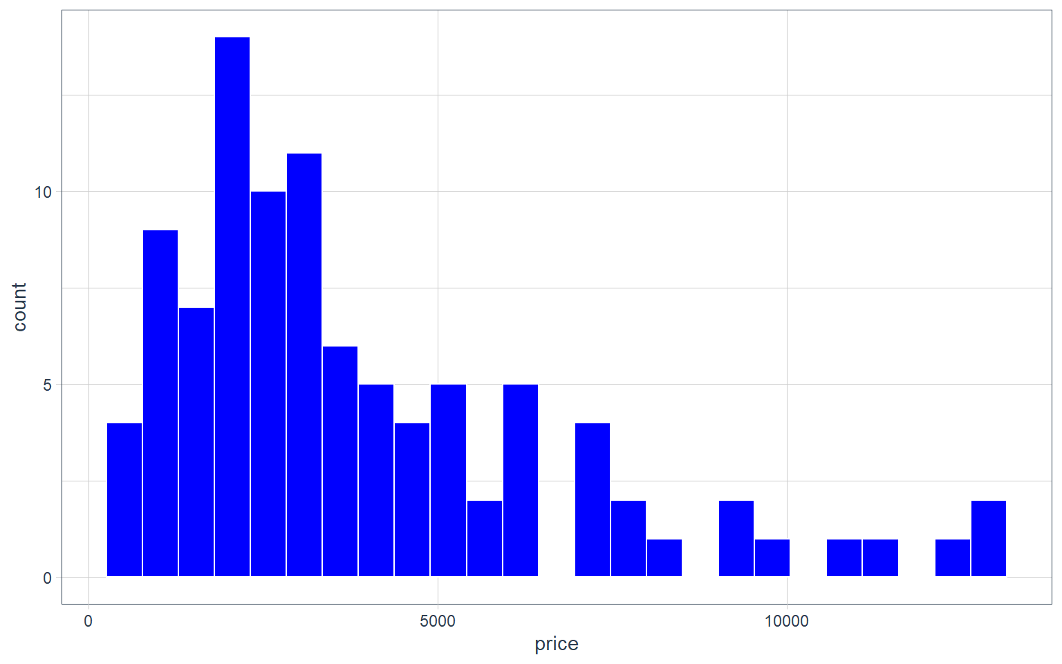
Unit price of bicycle, segmenting by frame material
# Histogram
bike_orderlines_tbl %>%
  distinct(price, model, frame_material) %>%
  ggplot(mapping = aes(x = price, fill = frame_material)) +
  geom_histogram() +
  facet_wrap(~ frame_material, ncol = 1) +
  tidyquant::theme_tq() +
  tidyquant::scale_fill_tq() +
  theme_classic()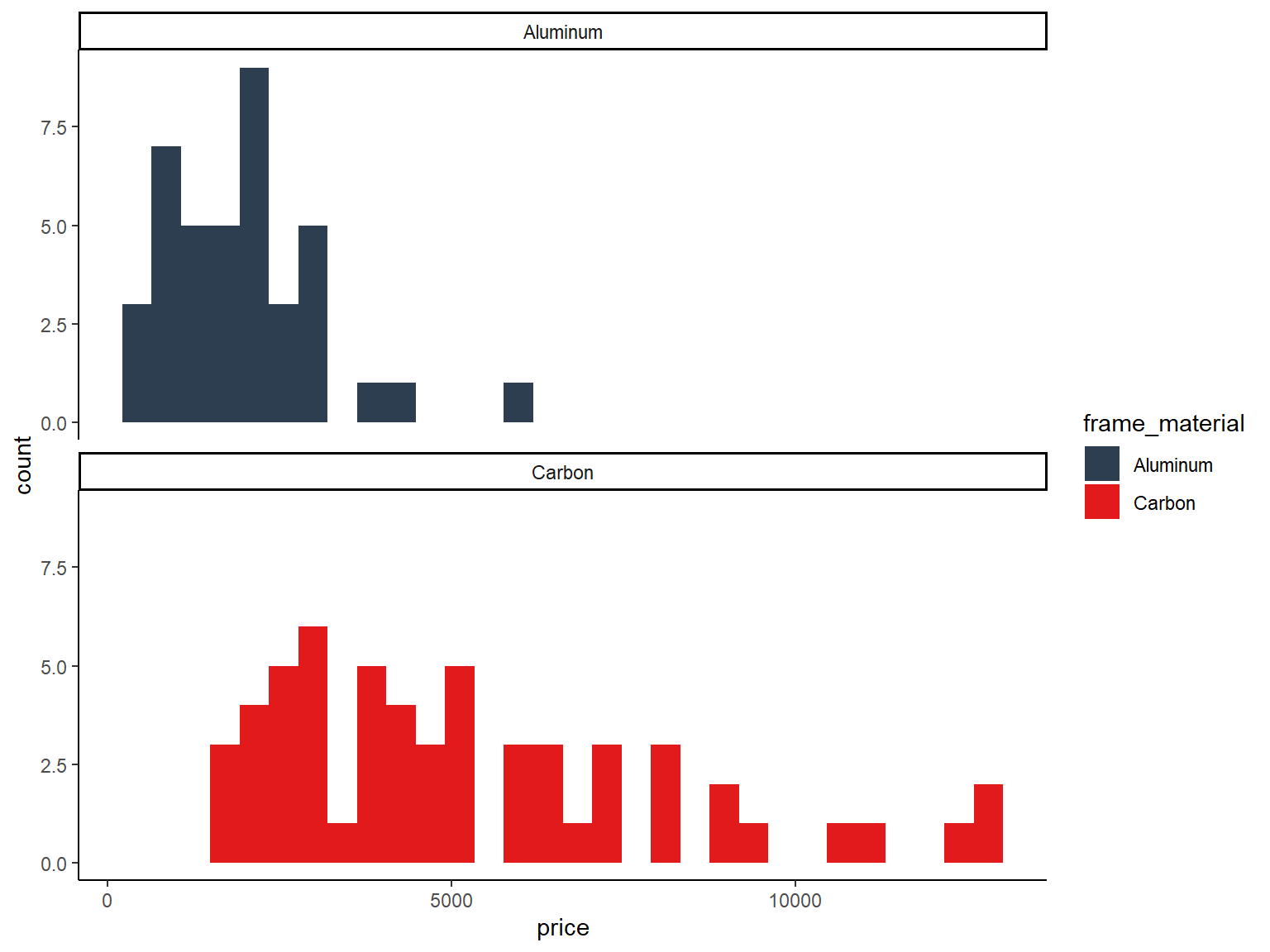
# Density
bike_orderlines_tbl %>%
  distinct(price, model, frame_material) %>%
  ggplot(mapping = aes(x = price, fill = frame_material)) +
  geom_density(alpha = 0.618) +
  tidyquant::scale_fill_tq() +
  tidyquant::theme_tq()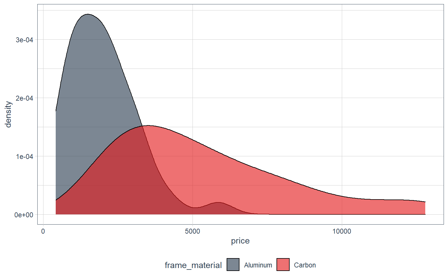
Unit price of models, segmenting by secondary category
# Box Plot / Violin Plot (Comparing distributions)

# Data Manipulation
unit_price_by_cat2_tbl <- bike_orderlines_tbl %>%
  distinct(category_2, model, price) %>%
  mutate(category_2 = category_2 %>% as_factor() %>% fct_reorder(price))

# Box Plot
unit_price_by_cat2_tbl %>%
  ggplot(mapping = aes(x = category_2, y = price)) +
  geom_boxplot() +
  coord_flip() +
  tidyquant::theme_tq()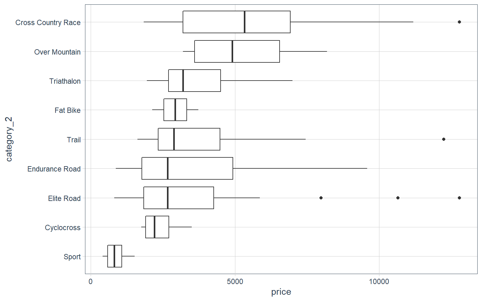
# Violin Plot & Jitter Plot
unit_price_by_cat2_tbl %>%
  ggplot(mapping = aes(x = category_2, y = price)) +
  geom_violin() +
  geom_jitter(width = 0.2, color = "#2c3e50") +
  coord_flip() +
  tidyquant::theme_tq()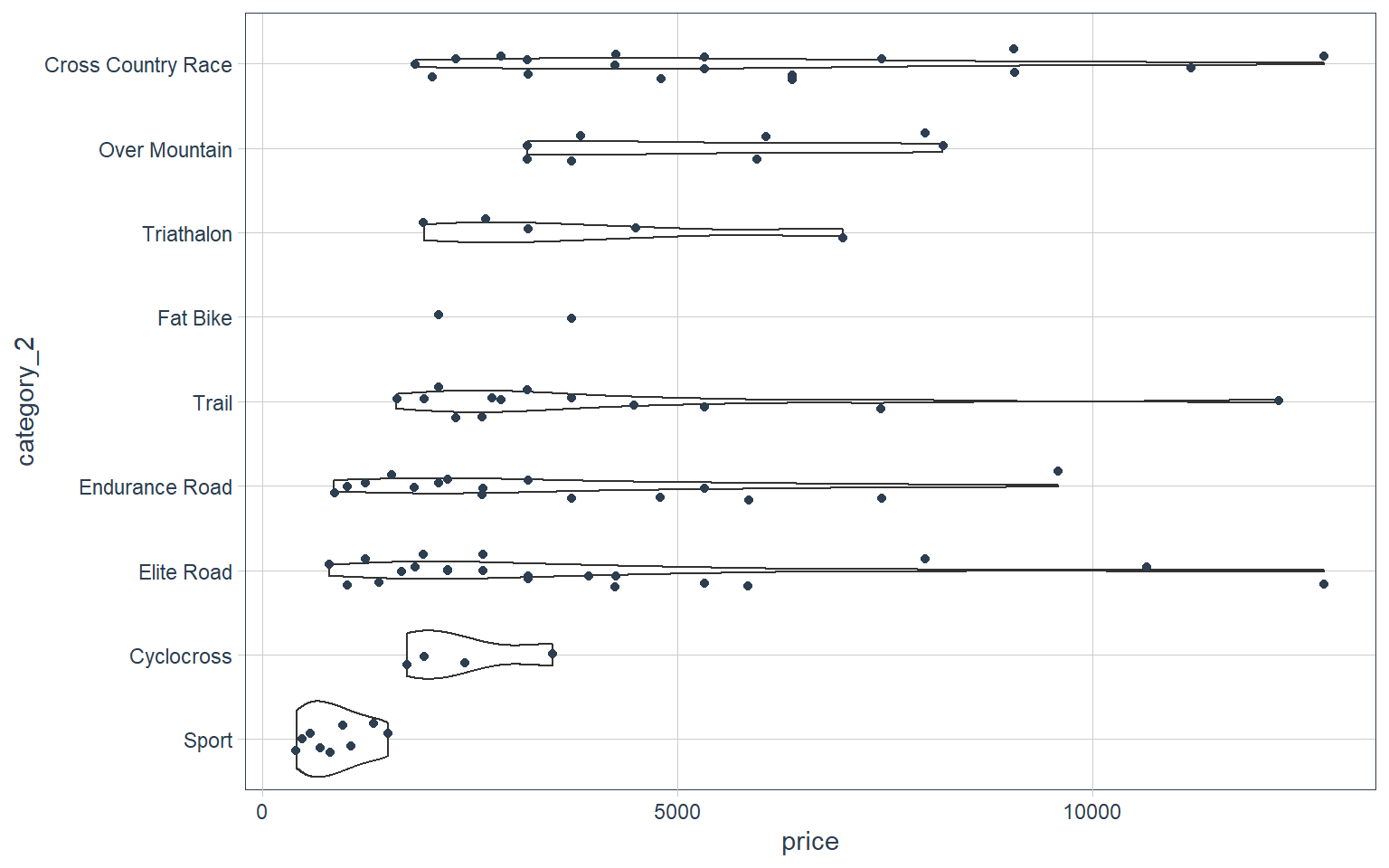
Top Customers
How much purchasing power is in top 5 customers?
Visualize top N customers in terms of Revenue, include cumulative percentage
n <- 15

# Data Manipulation
top_customers_tbl <- bike_orderlines_tbl %>%
  select(bikeshop_name, total_price) %>%
  mutate(bikeshop_name = bikeshop_name %>% as_factor() %>% fct_lump(n = n, w = total_price)) %>%
  group_by(bikeshop_name) %>%
  summarise(revenue = sum(total_price)) %>%
  ungroup() %>%
  mutate(bikeshop_name = bikeshop_name %>% fct_reorder(revenue)) %>%
  mutate(bikeshop_name = bikeshop_name %>% fct_relevel("Other", after = 0)) %>%
  arrange(desc(bikeshop_name)) %>%
  # revenue text
  mutate(revenue_text = scales::dollar(revenue, scale = 1e-6, suffix = "M")) %>%
  # cumulative percent
  mutate(cum_pct = cumsum(revenue)/sum(revenue)) %>%
  mutate(cum_pct_text = scales::percent(cum_pct)) %>%
  # Get a rank
  mutate(rank = row_number()) %>%
   mutate(rank = case_when(
     rank == max(rank) ~ NA_integer_,
     TRUE ~ rank)) %>%
  # Label Text
  mutate(label_text = str_glue("Rank: {rank}\nRev: {revenue_text}\nCumPct: {cum_pct_text}"))


# Data Visualization
top_customers_tbl %>%
  ggplot(mapping = aes(x = revenue, y = bikeshop_name)) +
  geom_segment(mapping = aes(xend = 0, yend = bikeshop_name), color = palette_light()[1], size = 1) +
  geom_point(color = palette_light()[1], mapping = aes(size = revenue)) +
  geom_label(mapping = aes(label = label_text), hjust = "inward", size = 3, color = palette_light()[1]) +
  # Formatting
  scale_x_continuous(labels = scales::dollar_format(scale = 1e-6, suffix = "M")) +
  labs(title = str_glue("Top {n} Customers"), subtitle = str_glue("Start: {year(min(bike_orderlines_tbl$order_date))}
                                                                  End:  {year(max(bike_orderlines_tbl$order_date))}"),
       x = "Revenue ($M)",
       y = "Customer",
       caption = str_glue("Top 6 customers contribute 51% of purchasing power")) +
  theme_tq() +
  theme(legend.position = "none", plot.title = element_text(face = "bold"),
        plot.caption = element_text(face = "bold"))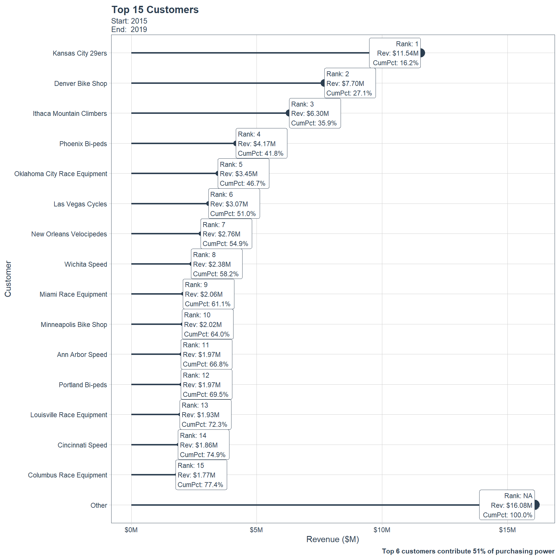
Do specific customers have a purchasing preference?
Marketing would like to increase email campaign engagement by segmenting the customer-base using their buying habits.
Customer Trends: Customer purchase history for similarity to other “like” customers.
Customer preferences
Our customer-base consists of 30 bike shops. Several customers have purchasing preferences for Road or Mountain Bikes based on the proportion of bikes purchased by category_1 and category_2.
Heatmap of proportion of sales by secondary product category
# Data Manipulation
pct_sales_by_customer_tbl <- bike_orderlines_tbl %>%
    select(bikeshop_name, category_1, category_2, quantity) %>%
    group_by(bikeshop_name, category_1, category_2) %>%
    summarise(total_quantity = sum(quantity, na.rm = TRUE)) %>%
    ungroup() %>%
    group_by(bikeshop_name) %>%
    mutate(pct = total_quantity/sum(total_quantity, na.rm = TRUE)) %>%
    ungroup() %>%
    # List shops by alpha
    mutate(bikeshop_name = as.factor(bikeshop_name) %>% fct_rev()) %>%
    #mutate(bikeshop_name_num = bikeshop_name %>% as.numeric()) %>%
    mutate(label_text = str_glue("Customer: {bikeshop_name}
                                     Category = {category_1}
                                     Sub-Category = {category_2}
                                     Quantity Purchased: {total_quantity}
                                     Percent of Sales: {scales::percent(pct)}"))

# Data Visualization
g <- pct_sales_by_customer_tbl %>%
  ggplot(
    mapping = aes(x = category_2, y = bikeshop_name)) +

  # Geometries
  geom_tile(
    mapping = aes(fill = pct)) +
  geom_text(
    mapping = aes(
      label = scales::percent(pct, accuracy = .01),
      text = label_text), size = 3) +
  facet_wrap(~ category_1, scales = "free_x") +

  # Formatting
  scale_fill_gradient(low = "white", high = palette_light()[1]) +
  labs(
    title = "Heatmap of Purchasing Habits",
    x = "", #Bike Type (Cateogry 2)
    y = "", #Customer
    caption = str_glue("Customers that prefer Road: Ann Arbor Speed, Austin Cruisers, & Indianapolis Velocipedes
                        Customers that prefer Mountain: Ithica Mountain Climbers, Pittsburgh Mountain Machines, & Tampa 29ers")) +
  theme_tq() +
  theme(
    legend.position = "none",
    axis.text.x = element_text(angle = 45, hjust = 1),
    plot.caption = element_text(face = "bold.italic"),
    plot.title = element_text(face = "bold"))
   # strip.text.x = element_text(margin = margin(5,5,5,5, unit = "pt")))


ggplotly(g, tooltip = "text")
Order vs Quantity
Explain relationship between order value and quantity of bikes sold.
# - Continuous vs Continuous

# Explain relationship between order value and quantity of bikes sold

# Data Manipulation
order_value_tbl <- bike_orderlines_tbl %>%
  select(order_id, order_line, total_price, quantity) %>%
  group_by(order_id) %>%
  summarize(
    total_quantity = sum(quantity),
    total_price = sum(total_price)) %>%
  ungroup()

# Scatter Plot
order_value_tbl %>%
  ggplot(
    mapping = aes(
      x = total_quantity, y = total_price)) +
  geom_point(alpha = 0.312, position = "jitter", size = 2) +
  geom_smooth(method = "lm", se = F) +
  theme_classic()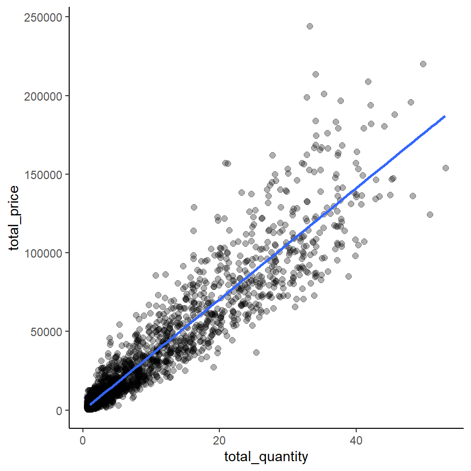
Customer Segmentation
This is a 2D Projection based on customer similarity that exposes 4 clusters, which are key segments in the customer base.
Interactive Clusters
# Plot customer segments
plot_customer_segments(interactive = interactive, k = 4, seed = 123)
Static Labeled Clusters
# Plot customer segments
plot_customer_segments(interactive = FALSE, k = 4, seed = 123)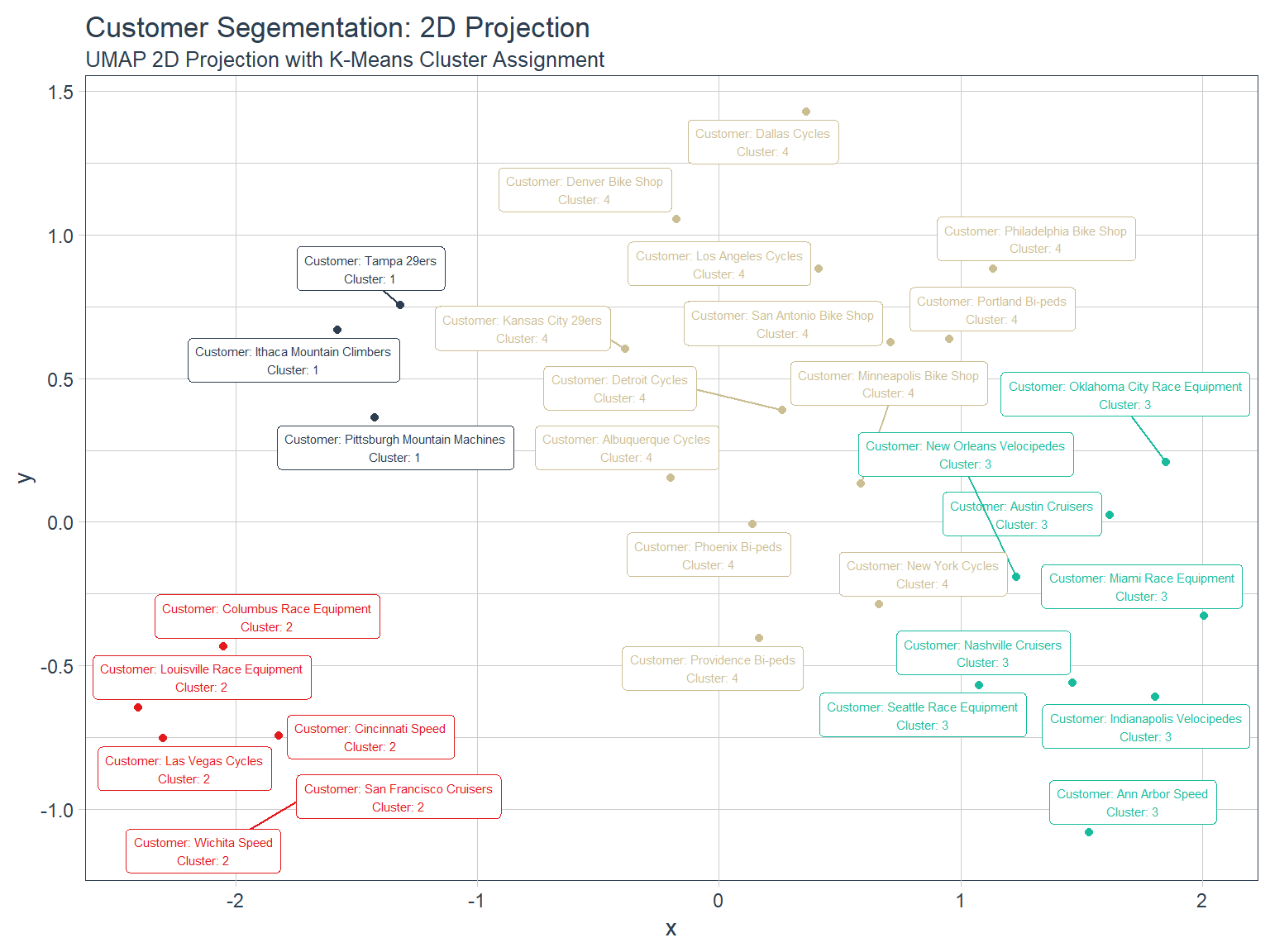
Customer Preferences By Segment
The 4 customer segments were given descriptions based on the customer’s top product purchases.
Segment 1 Preferences: Mountain Bikes, Above $3k
Segment 2 Preferences: Road Bikes, Above $3k
Segment 3 Preferences: Road Bikes, Below $3k
Segment 4 Preferences: Mountain Bikes, Below $3k
plot_customer_behavior_by_cluster(interactive = interactive, top_n_products = 10, k = 4, seed = 123)